


Abstract
Spectral induced polarization measurements are affected by temperature variations due to a variety of temperature-dependent parameters that control the complex electrical conductivity. Most important is the influence of the ion mobility, which increases with increasing temperature. It is responsible for the increase of the conductivity of the fluid in the pores with temperature and influences the electrical double layer on the mineral surface. This work is based on laboratory measurements of 13 sandstone samples from different sources with different geological and petrophysical characteristics. We measured the complex impedance in a frequency range from 0.01 to 100 Hz and a temperature range from 0 to 40 °C. The main observation is a decrease of the characteristic time (defined by the inverse of the frequency, at which the phase shift is maximum) with increasing temperature. The strength of this decrease differs from one sample to another. The temperature dependence of the phase shift magnitude cannot easily be generalized, as it depends on the particular sample. The experimental findings suggest that neglecting the influence of temperature on complex conductivity may lead to significant errors when estimating hydraulic conductivity from relaxation time. We also simulate the temperature dependence with a theoretical model of membrane polarization and review some of the model properties, with an emphasis on the temperature dependence of the parameters. The model reproduces several features characterizing the measured data, including the temperature dependence of the characteristic times. Computed tomography and microscope images of the pore structure of three samples also allow us to associate differences in the geometrical parameters used in the modelling with pore scale parameters of the actual samples.
1 INTRODUCTION
The complex electrical conductivity of sediments is influenced by different physical properties, including the temperature. Consequently, variations of the temperature of the subsurface may change the results of induced polarization (IP) measurements in the field. Seasonal and weather-related differences in temperature may lead to notable variations particularly for the shallow subsurface, and measurement results might not be comparable if taken at different temperatures. Relations between IP parameters and petrophysical or hydrological parameters are often based on laboratory measurements, which are usually performed at room temperature or in climate chambers. The typical temperature is around 25 °C, which does not necessarily coincide with the ambient temperature of the subsurface under in situ conditions. The differences in temperature near the surface are usually small, but it is also conceivable that induced polarization measurements may be used for exploration of geothermal areas, where a large temperature range is covered, as IP is particularly suitable for estimating the hydraulic conductivity of the subsurface (e.g. Börner et al.1996; Hördt et al.2007).
The temperature dependence of DC conductivity was studied by several authors, using various physical and empirical approaches (e.g. Llera et al.1990; Sen & Goode 1992; Hayley et al.2007) and is well known. However, there is a number of temperature-dependent parameters, which influence the complex frequency-dependent electrical conductivity additionally to the DC conductivity of porous media. The complex electrical conductivity increases with increasing temperature, both in the real and imaginary part, as reported, for example, in Binley et al. (2010) for temperatures between 5 and 30 °C. The time constant decreases with increasing temperature as a consequence of increasing ion mobility. This is described for timescales determined from the inverse of the spectral position of the phase maximum (Binley et al.2010) and for mean relaxation times from a Debye decomposition (Zisser et al.2010a) and also by Tong & Tao (2007) for IP measurements in the time domain. Tong & Tao (2007) also proposed a correction of temperature effects on the relaxation time of shaly sands by shifting the relaxation time spectra along the relaxation time axis.
Observations of measured parameters describing the polarization strength differ depending on the investigated material. Collett (1959) reported an increase of the polarization strength of andesite particles with increasing temperature for clean material, but a decrease if a small amount of pyrite is added. A similar relation was found by Vinegar & Waxman (1984) for a sandstone sample with low clay content compared to a sandstone sample with high clay content for temperatures between −5 and 95 °C. An influence of the clay content on the temperature dependence was observed also by Treichel et al. (2014). However, the phase shift of the sandstone samples investigated by Binley et al. (2010) remained constant. Worthington & Collar (1984) refer to measurements of other authors, who observed a change in the polarization with temperature that was not monotonous.
Although there are several investigations of the temperature dependence of spectral induced polarization (SIP), the existing data comprise only a few different sample materials and some of the observations differ. Especially, the behaviour of the phase shift is poorly constrained. Moreover, it is unclear if conclusions made on observations of individual samples are valid also for other materials.
The theoretical background of the temperature dependence of the complex electrical conductivity is based mainly on empirical or semi-empirical approaches, which do not cover all characteristics of the measured data. An approach to explain the temperature dependence of the phase shift can be found in Revil (2012), who describes the influence of temperature on SIP with different temperature dependencies of the ion mobilities in the free electrolyte, the diffuse layer and the Stern layer of the electrical double layer (EDL). However, a general conclusion about the temperature behaviour is not suggested.
Temperature-dependent SIP data may also be useful to test existing theories about the origin of the IP effect, including mechanistic models. Mechanistic models in turn provide a good opportunity to improve our understanding of the temperature dependence of the polarization effects in porous media. Furthermore, models can help to generalize the observations of measurements and predict the temperature dependence of SIP data.
Currently, there are principally two types of models, which describe polarization mechanisms at the pore scale; the grain-based electrochemical polarization model (e.g. Schwarz 1962; Leroy et al.2008; Revil & Florsch 2010) and the pore-based membrane polarization model (e.g. Marshall & Madden 1959; Buchheim & Irmer 1979; Titov et al.2002). The membrane polarization model, suggested by Marshall & Madden (1959), solves the equations describing the motion of ions for a 1-D geometry. Changing ion mobilities along the pore system leads to a concentration gradient, when an external electric field is applied. Bücker & Hördt (2013a) extended this model by explicitly parametrizing the EDL and the pore radii of cylindrical pores.
In order to gain further insight into the temperature dependence of SIP, we add additional data acquired with different materials and compare them with previous observations and empirical relationships. We discuss the extended membrane polarization model by Bücker & Hördt (2013a) with an emphasis on the temperature dependence of the model parameters and compare measured with calculated phase spectra.
2 TEMPERATURE DEPENDENCE OF THE COMPLEX ELECTRICAL CONDUCTIVITY
There are two main factors causing the temperature dependence of the polarization response: (1) the electrical conductivity of the pore fluid, the temperature dependence of which basically stems from changes in ion mobility and (2) the EDL, coating the surface of the rock matrix or grains. The surface of the solid phase usually acquires a negative charge, when brought into contact with the pore fluid. Close to the surface within the electrolyte, the net surface charge results in an increased concentration of ions of opposite charge (counter ions). This region is known as the EDL, which consists of two parts; an inner Stern layer of strongly bound counter ions and an outer diffuse layer. Within the diffuse layer, ions can move freely but are affected by diffusion and electrostatic forces. The properties of the EDL are mainly controlled by the temperature-dependent parameters ion mobility, Zeta potential and Debye length.
The effect of the temperature dependence of Debye length and Zeta potential on the complex electrical conductivity will be discussed in the context of a membrane polarization model.
3 EXPERIMENTAL DATA
Measurements were carried out on 13 different sandstone samples (see Table 1). Samples TU-B1, TU-B4 and TU-B5 stem from different drilling cores obtained at the Ketzin pilot site, Germany, (e.g. Fleury et al.2013; Martens et al.2013, 2014) and sample P8 is a Bunter sandstone from an outcrop in the eastern Thuringian Basin. Samples BeRo1, Biu1, FrUK1, GiUK1, koQ1, koVe1, OK1 and smVG1 are sandstones from different outcrops at the North German Basin (see Reyer & Philipp (2014) for more details). Sample S3 is an Elb Sandstone, which was previously investigated by Hördt & Milde (2012) in a different context. All samples were cut into cylinders with a diameter of 25 mm and a length of 50 mm. Available geological and petrophysical parameters of the samples are listed in Table 1. The porosities were determined from the dry and saturated weight and the volume of the samples. Dominant pore-throat diameters and the surface-area/pore-volume ratio were measured by mercury injection and nitrogen adsorption, respectively.
Geological and petrophysical parameters of the sandstone samples. Parameters listed are: porosity Φ, pore-fluid conductivity σf at 20 °C, dominant pore-throat radius rdom, mean grain size d, specific surface area Spor, clay content, mineralogy, cementation c, sorting s and rounding r.
| Sample | Local name | Φ | σf | rdom | d | Spor | Clay | Mineralogy | c | sc | rc |
|---|---|---|---|---|---|---|---|---|---|---|---|
| [ per cent] | [mS m−1] | [μm] | [μm] | [1 μm−1] | [ per cent] | [ per cent] | [ per cent] | ||||
| TU-B1 | Stuttgart Fm. | 27.5 | 47.9 | 9.1 | 90 | 116.6 | 16.0 ± 10.4a | 36.6 ± 6.1 Q, 21.8 ± 4.6 Fa | – | – | – |
| TU-B4 | Exter Fm. | 21.3 | 53.8 | 0.7 | – | 147.1 | – | – | – | – | – |
| TU-B5 | Exter Fm. | 17.0 | 55.4 | 2.8 | 210 | 213.6 | – | – | – | – | – |
| P8 | Bunter Sst. | 11.2 | 34.2 | 1.4 | 180 | 47.2 | – | – | – | – | – |
| BeRo1 | Rotliegend Sst. | 6.9 | 64.6 | 6.0 | 400 | 64.9 | 3.3b | 59.1 Q, 4.2 F, 36.7 Lb | 17.6b | 4 | 2.5 |
| BiSu1 | Bernburg-F. | 19.8 | 54.4 | 6.4 | 210 | 20.3 | 0.9b | 72.2 Q, 17.1 F, 10.7 Lb | 12.3b | 2 | 3 |
| FrUK1 | Bentheimer Sst. | 14.6 | 57.4 | 5.9 | 100 | 46.6 | 4.3b | 96.1 Q, 2.1 F, 1.8 Lb | 17.0b | 3.5 | 3.5 |
| GiUK1 | Gildehaus Sst. | 22.7 | 54.9 | 16.8 | 250 | 1.8 | 1.3b | 94.9 Q, 2.4 F, 2.7 L | 16.8 | 2 | 2.5 |
| koQ1 | Rhät Sst. | 17.1 | 56.9 | 9.7 | 200 | 20.6 | 0.0b | 78.6 Q, 4.7 F, 16.7 Lb | 31.0b | 1 | 3 |
| koVe1 | Rhät Sst. | 13.0 | 60.6 | 0.9 | 100 | 96.8 | 0.0b | 83.2 Q, 3.8 F, 13.0 Lb | 40.0b | 1 | 3 |
| OK1 | Wealden Sst. | 18.9 | 58.4 | 1.5 | 200 | 14.6 | 2.8b | 94.2 Q, 4.0 F, 1.8 Lb | 17.4b | 2 | 3 |
| smVG1 | Volpriehausen-F. | 20.1 | 46.6 | 5.3 | 210 | 11.3 | 0.8b | 80.1 Q, 15.8 F, 4.1 Lb | 23.8b | 3.5 | 3 |
| S3 | Elb Sst. | 19.3 | 54.8 | 22.2 | 330 | 9.7 | – | – | – | – | – |
For three investigated rock samples (TU-B1, P8 and S3) X-ray computed tomography (CT) scans could be obtained using a GE phoenix nanotom® s system. The CT scans of these sandstone samples were acquired on small pieces of a few millimetres in diameter. The resolution of the scans was 1.25 μm (sample TU-B1), 1.5 μm (sample P8) and 2.0 μm (sample S3), respectively. 2-D images of the scans of the sandstone samples are shown in Fig. 1.
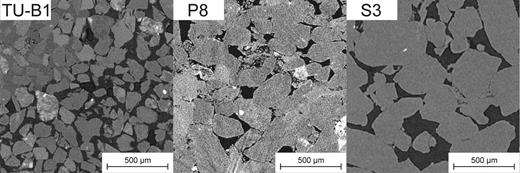
2-D images of computed tomography (CT) scans of the pore space of three investigated samples. Left: sample TU-B1. Middle: sample P8. Right: sample S3.
The main differences between the three sandstone samples are: (1) the size of the grains is smallest for sample TU-B1 and largest for S3. The grains of P8 and S3 are more rounded than the grains of TU-B1. (2) Samples P8 and S3 are more consolidated and compacted than TU-B1. The visually higher compaction is consistent with the lower porosity of sample P8 and S3 (0.11 and 0.19, for comparison: TU-B1 0.27), and the fact that P8 and S3 are robust while TU-B1 is brittle. Due to the different degrees of consolidation we assume that the pores of TU-B1 are wider than those of P8. The CT image shows that sample S3 has large pores compared to P8. This assumption is supported by mercury injection measurements, which reveal dominant pore-throat diameters of 18.3 μm for TU-B1, 2.9 μm for sample P8 and 44.4 μm for sample S3 (Table 1). However, sandstone samples TU-B1 and P8 are inhomogeneous and show regions with high cementation, where much smaller pores may exist. For estimating the pore length, we refer to the mean grain size, which is approximately 180 and 330 μm for P8 and S3, respectively (see Table 1). Because of the weak consolidation of sample TU-B1 we assume that the pores are longer than the mean grain size and similar to the length of sample P8.
3.1 SIP measurements
SIP measurements were performed with a VMP3 impedance analyser by Princeton Applied Research in the frequency range of 0.01–100 Hz. We used four-point measuring cells with non-polarizing potential electrodes as described in detail by Kruschwitz (2008), Hördt & Milde (2012) and Bairlein et al. (2014). The filled measuring cell was stored within a climate chamber with an accuracy of 0.1 °C to keep the temperature of the sample at the desired value. In order to assess the accuracy of the current measuring system, the measuring cell was filled with a sodium chloride solution (σF(20 °C) = 50,0 mS m−1) and measurements at temperatures between 0 and 90 °C were carried out. Fig. 2 shows that the measured electrical conductivity coincides with the increase of water conductivity with increasing temperature as predicted by the modified Walden product (eq. 2) for αμ = 0.91 and T0 = 25 °C. This observation is independent of frequency. The measured phase shift is zero with a standard deviation of 0.2 mrad (not shown here for brevity) for frequencies between 1 mHz and 10 Hz. During the measurements, particularly at high temperatures, a small amount of water (a few millilitres) evaporated through narrow chinks between the individual parts of the sample holder, which led to a slight increase of fluid conductivity to σF(20 °C) = 54,9 mS m−1 by the end of this test. Due to this change in fluid conductivity αμ might be slightly overestimated, but it is still in the range between 0.8 and 0.97 given by Zisser et al. (2010a).
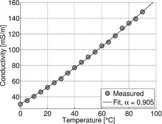
Magnitude of the electrical conductivity at 1 Hz versus temperature for a water-filled sample holder (circles) fitted with eq. (2) and ασ = 0.905 (solid line). The fluid conductivity at 20 °C increased during the measurement series from 50.0 to 54.9 mS m−1.
Before the actual measurements, the rock samples were dried in a vacuum chamber at 30 °C for at least 48 hr to remove residual water from the pores. Afterwards, the samples were saturated with a sodium chloride solution. The saturation process was performed slowly and under vacuum conditions in order to avoid air being trapped inside the pores. After saturation, the sample and the fluid had to equilibrate, which took several days, differing from one sample to another. When water conductivity had remained constant for at least two days, the sample was inserted into the sample holder. At the time of the measurements, the ion concentration had increased, most probably due to the dissolution of salt that precipitated during the drying procedure and/or the dissolution of ions from the mineral matrix of the samples. Pore fluid conductivities of the samples taken before the SIP measurements are listed in Table 1.
Temperature was increased from 0 to 40 °C in steps of 5 °C. The time between increasing the temperature and starting the measurement was at least 24 hr to ensure that the sample was at the required temperature and chemical equilibrium during the measurement. Tests showed that the major change in conductivity occurred within the first two hours after a temperature change of 5 °C. Before each of these measurement series from 0 to 40 °C, one reference measurement at 20 °C was performed to assess any change of the measured spectra with time. A comparison of the reference spectra with those taken at 20 °C during the measurement series shows a slight change of electrical conductivity with time, which is supposed to arise from ions dissolved during the measurement series. The real part of the conductivity at 20 °C increases stronger during the measurements series than the imaginary part, resulting in a slight decrease of the phase shift with time.
Both real and imaginary part of the electrical conductivity increase with temperature, shown exemplarily for sample TU-B1 in Fig. 3. In agreement with eq. (1), the real part increases linearly by about 2 per cent per °C regardless of the frequency. The temperature increase of the imaginary part though depends on frequency. Its increase is largest (2.4 per cent per K for sample TU-B1) at the peak frequency fpeak, where the maximum of the imaginary conductivity can be observed, and smallest (1.9 per cent per K) at 0.01 Hz, where the phase shift is smallest. The different temperature dependencies of real and imaginary conductivity result in slight changes in the phase shift with temperature.
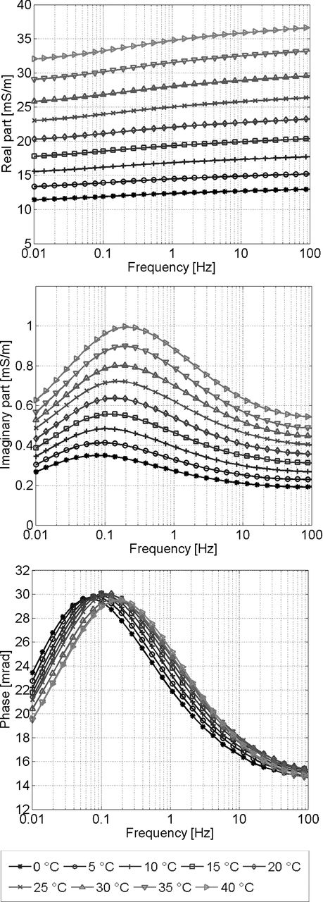
Real part (top), imaginary part (middle) and phase shift (bottom) of the electrical conductivity of sandstone sample TU-B1 for temperatures from 0 to 40 °C.
The temperature dependence of the real part of conductivity can be described quantitatively by fitting eq. (2) to the data. The Walden exponents ασ presented in Table 2 are determined from the real conductivity at 1 Hz, which is typically used for evaluating SIP data at a single frequency (e.g. Weller et al.2010). As stated before, for the real part of conductivity, the temperature dependence is independent of frequency. Most of the values are in the range previously reported in literature. Some of the samples exhibit stronger temperature dependencies (ασ > 1). Exponents > 1 mean that temperature-dependent parameters other than ion mobility become important. One possible explanation is that surface conductivity, which also depends on Zeta potential and the EDL thickness, becomes important.
Characteristic times τpeak at 25 °C and Walden exponents obtained from fitting eqs (2) and (6) to the temperature dependence of the real conductivity ασ and the characteristic times ατ, respectively, along with standard deviations δα of the fits. Tmax is the temperature, where the phase peak is largest within the temperature range of 0–40 °C. Sample FrUK1 does not show a maximum phase shift in the investigated frequency range.
| Sample | ασ | δ ασ | τpeak(25 °C) [s] | ατ | δ ατ | Tmax [°C] |
|---|---|---|---|---|---|---|
| TU-B1 | 0.98 | 0.00 | 1.24 | 0.81 | 0.04 | 20 |
| TU-B4 | 1.05 | 0.01 | 0.45 | 0.75 | 0.14 | 40 |
| TU-B5 | 1.02 | 0.02 | 0.34 | 0.52 | 0.06 | 0 |
| P8 | 1.13 | 0.01 | 0.52 | 0.92 | 0.16 | 0 |
| BeRo1 | 1.07 | 0.00 | 1.99 | 1.30 | 0.29 | 15 |
| BiSu1 | 0.95 | 0.01 | 0.23 | 0.91 | 0.07 | 10 |
| FrUK1 | 0.85 | 0.03 | – | – | – | – |
| GiUK1 | 0.87 | 0.01 | 4.12 | 0.92 | 0.15 | 30 |
| koQ1 | 0.85 | 0.01 | 0.35 | 0.72 | 0.15 | 40 |
| koVe1 | 0.93 | 0.01 | 0.84 | 1.42 | 0.13 | 40 |
| OK1 | 0.97 | 0.00 | 0.71 | 0.83 | 0.08 | 40 |
| smVG1 | 0.86 | 0.00 | 0.18 | 0.68 | 0.08 | 40 |
| S3 | 0.88 | 0.02 | 3.83 | 0.89 | 0.06 | 35 |
The phase spectra of six of the investigated samples are displayed in Fig. 4. A common feature of the phase spectra is the increase of the frequency of the maximum phase shift with temperature, that is, the spectra shift towards higher frequencies. This is particularly obvious for all samples except GiUK1. Also the samples not presented in Fig. 3 show this behaviour. The phase spectra of sample GiUK1 appear a bit more noisy, because the phase shifts are much smaller (max. 4.5 mrad compared to up to 30 mrad for the others). Sample GiUK1 is also the only sample, which exhibits two phase maxima. While the low-frequency maximum shifts towards higher frequencies with temperature, which is in agreement with the other four samples. The high-frequency maximum appears to be independent of frequency, which might be caused by the overlay of electromagnetic coupling effects.
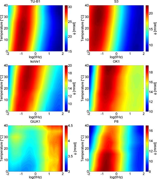
Phase shift of the electrical conductivity colour coded versus temperature and frequency of samples TU-B1, S3, koVe1, OK1 and GiUK and P8. Note that the colour scales are different.
In order to quantify the shift towards higher frequencies and compare it with theoretical predictions, we calculated a characteristic time as the inverse of the frequency where the maximum phase shift occurs (τpeak = (2πfpeak)−1) (Fig. 5). The peak frequencies fpeak were determined with the help of a spline interpolation between the measured frequencies. The characteristic times decrease with increasing temperature and can be fitted with eq. (6) and Walden exponents listed in Table 2. To reduce the effect due to the error of the characteristic time at the reference temperature τ(T0), we used every measured temperature as reference temperature to realize a separate fit. The final Walden exponents are the averages of these separate realizations along with the corresponding standard deviations δαtau (Table 2). The exponents αtau range from 0.52 to 1.42, which is a wider range than the values reported in literature (0.8–0.97). Compared to the real part of conductivity, the characteristic times show a wider variation in temperature dependence and also values ατ that are significantly smaller than the temperature dependence of fluid conductivity (αμ = 0.905). For some of the samples the standard deviations of the fits δαtau are large, resulting from the scatter in the characteristic times, that may arise from the precision of the phase shift of 0.2 mrad.
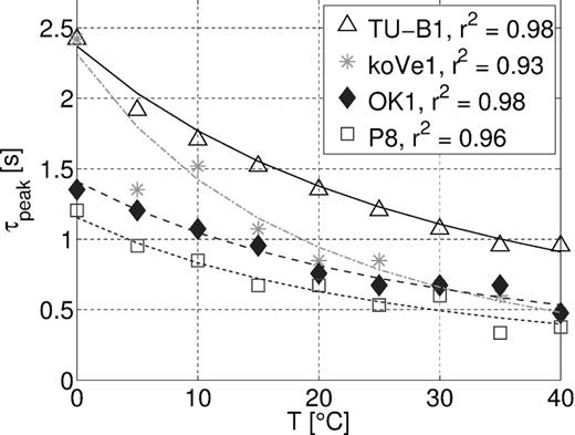
The temperature dependencies of the amplitude of the maximum phase shifts (Fig. 4) are less uniform (i.e. the maximum phase shift can either increase or decrease with temperature) than the characteristic times. While the phase spectra of samples TU-B1, S3 and GiUK1 show an absolute maximum at 20, 35 and 30 °C, respectively, the maximum phase shift of samples koVe1 and OK1 slightly increases over the entire temperature range, indicating an absolute maximum at higher temperatures. The maximum phase shift of sample P8 decreases with increasing temperature, indicating an absolute maximum that is shifted to smaller temperatures compared to samples TU-B1, S3 and GiUK1. The temperatures of the absolute maximum in the phase shift Tmax of all samples are listed in Table 2.
In order to analyse the cause of the differences in the temperature dependence of different samples, we examined if there is any correlation to the sample characteristics. It seems natural that the influence of the EDL gets stronger with decreasing pore diameter, thus the Walden exponents of samples with small dominant pore-throat radius rdom should deviate stronger from the Walden exponent of the electrolyte (α = 0.91) than the exponents of samples with large pores. The temperature dependence of the real part of conductivity versus rdom (Fig. 6) suggests a weak correlation of both parameters rdom and ασ, but the poor coefficient of determination (r2 = 0.29) indicates that also other parameters have a strong influence. For the Walden exponents of the characteristic times, no correlation with rdom could be observed. Possibly, rdom is too simplified to characterize the pore space sufficiently and the entire pore- (or grain) size distribution needs to be taken into account. For none of the remaining parameters in Table 1, we could find a direct correlation to the temperature dependence of ασ or ατ. However, we cannot exclude that a combination of surface characteristics and the geometry of the pore space determines the temperature dependence.
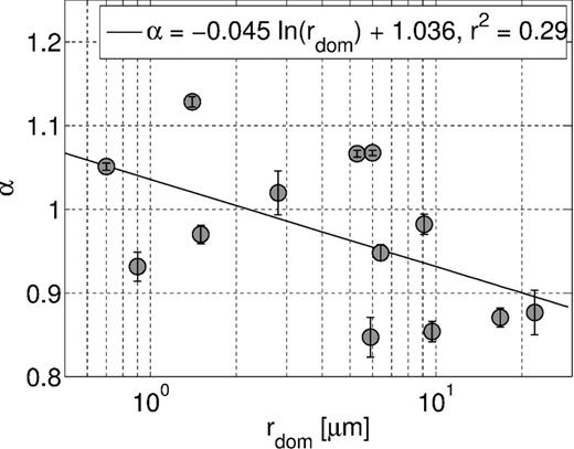
Walden exponent of the real conductivity versus dominant pore-throat diameter. The solid line corresponds to the logarithmic fit.
4 MODELLING THE TEMPERATURE DEPENDENCE
Our experimental results suggest that the temperature dependence of SIP data cannot be explained solely by the temperature dependence of ion mobilities. In order to obtain a deeper theoretical understanding, we carry out simulations with an existing membrane polarization model that allows to simulate temperature dependence, including the EDL properties. While we do not expect to obtain a quantitative fit to the data, we hope to be able to explain at least some of the observations with processes at the pore scale.
4.1 Membrane polarization model
The original model by Marshall & Madden (1959) was designed to roughly estimate the magnitude of possible membrane polarization processes. The authors postulated the required mobility variations along the pores without suggesting a mechanism or quantitative estimates. Therefore, Bücker & Hördt (2013a) explicitly attributed the ion-selective behaviour of the active zone to the EDL, which coats the solid–fluid interface of porous media. In the following, we briefly review their model with an emphasis on the temperature dependence. The model describes the pore space as a sequence of wide and narrow cylindrical pores and allows to include pore radii and the properties of the EDL explicitly into the original membrane polarization model.
4.2 Modelling results
In order to explore how the overall polarization process responds to the temperature dependencies of the different model parameters described above, we carry out a modelling study. If no other value is specified, the following model parameters will be used: pore lengths are chosen to fit the typical pore size of a fine-grained sandstone (e.g. Howard et al.1993; Lindquist et al.2000; Peng et al.2012) with the length of the wide pore L1 = 50 μm and the length of the narrow pore L2 = 10 μm. Pore radii are chosen to cause a significant phase response of the model impedance (r1 = 0.2 μm and r2 = 0.02 μm for the wide pore and the narrow pore, respectively). The ion concentration of the pore fluid was set to 1 mol m−3. An ion mobility of |$5 \times \ 10^{-8} \frac{m^2}{Vs}$| was used, which is approximately the mobility of a Na+ ion (e.g. Atkins & De Paula 2013). Following Leroy et al. (2008), a Zeta potential of −75 mV and a (constant) partition coefficient of 0.6 were used. For calculating the ion mobility (eq. 3), we used a Walden exponent of αμ = 0.91, which was the best matching value for the data of Zisser et al. (2010a). The reference temperature T0 for the calculation of the temperature dependence of the mobilities and the Zeta potential (eq. 7) was 25 °C. The porosity for calculating the effective conductivity was Φ = 0.2, which is a typical value for sandstones.
For all frequencies in the range from 10 mHz to 100 Hz, the real part of the effective conductivity increases monotonously with temperature (Fig. 7). The modeled temperature dependence of the real part of the effective conductivity can be fitted by a Walden product (eq. 2) with an exponent ασ ≈ 2.19, which is large compared to the value that was chosen for the ion mobility in the free electrolyte (0.91). This large value implies, that the temperature dependence of the effective conductivity is strongly influenced by surface conductivity and cannot be described solely by the ion mobility in the free electrolyte. The temperature dependence of the surface conductivity is stronger than the dependence of the fluid conductivity on temperature. We conclude that besides the mobility other factors, most likely the Zeta potential and Debye length, also control the admittance. The conclusion is supported by the observation that the temperature dependence of the modeled real conductivity adopts the value of the mobility (0.91) for large pore radii (r1, r2 > 100 μm, not shown here for brevity) where the double layer becomes unimportant. The imaginary part of the effective conductivity also increases with temperature, depending on the frequency.
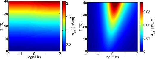
Effective conductivity of the model colour coded versus temperature and frequency calculated with parameters L1 = 50, L2 = 10, r1 = 0.2 and r2 = 0.02 μm. Left: real conductivity. Right: imaginary conductivity.
Fig. 8 shows the variation of the phase shift with frequency and temperature for three different pore lengths. The ratio of the two pore lengths L1 and L2 is kept constant, because it is more likely that in natural materials with long pores both narrow and wide pores are long compared to materials with short pores. The maximum phase shift attains highest values at medium temperatures (approximately 30 °C), which remain unchanged when the pore length is increased. Moreover, for all studied pore lengths, the peak frequency fpeak, where the maximum phase shift occurs, increases with increasing temperature. This translates into a decrease of the characteristic time (Fig. 9) with increasing temperature (calculated the same way as for the measured data), resulting mainly from the increase of ion mobility and diffusion coefficient as described by eq. (6). As reported before by Bücker & Hördt (2013a,b), the critical frequency of the membrane polarization model shifts towards lower frequencies, when increasing the pore length. Fitting the characteristic times with eq. (6) results in a slightly stronger temperature dependence of ατ = 1.07 than αμ = 0.91 used for the ion mobility. As for the admittance, mobility is not the only factor controlling the characteristic times.
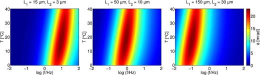
Phase shift of the modeled admittance colour coded versus temperature and frequency for different pore lengths L1 and L2. Pore lengths increase from left to right. Pore radii are r1 = 0.2 and r2 = 0.02 μm.
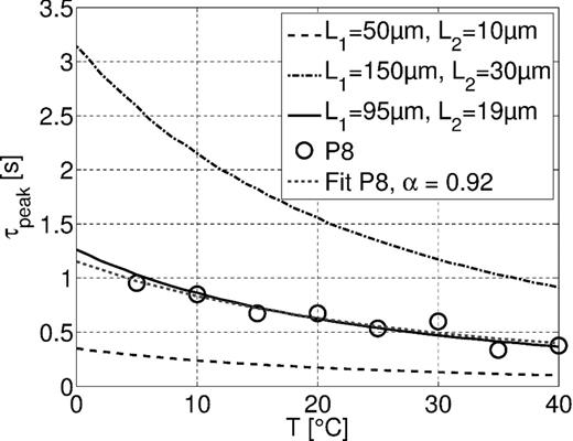
Modeled characteristic times of three different combinations of pore lengths L1 and L2 compared to the characteristic times of sample P8, fitted with ατ = 0.92. The pore radii are r1 = 0.2 and r2 = 0.02 μm.
Fig. 9 also shows that it is possible to fit the behaviour of the characteristic time of the data (using P8 as an example) almost exactly by choosing appropriate pore lengths. Measured and simulated curves of the characteristic times can be fitted with the modified Walden product with exponents of 0.92 (sample P8) and 1.07 (model).
Fig. 10 shows the variation of the phase shift with frequency and temperature for three different pore radii. Note that the ratio between the pore radii of the two pores is kept constant. Again, the peak frequency increases with temperature. Changing the pore radii in the range presented here has no influence on the characteristic timescale and its temperature dependence (not shown here). The absolute phase maximum though moves to higher temperatures when increasing pore radii, and changes its magnitude.
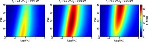
Phase shift of the modeled admittance colour coded versus temperature and frequency for different pore radii r1 and r2. Pore radii increase from left to right. Pore lengths are L1 = 50 and L2 = 10 μm.
5 DISCUSSION
Our measurement results exhibit a clear dependence of SIP parameters on temperature. The real part of the complex electrical conductivity of our measured IP spectra shows the expected increase of approximately 2 per cent per °C, which is in agreement with previous observations of other authors (e.g. Hayley et al.2007; Binley et al.2010). Similarly, the imaginary part increases about 2 per cent in average (consistent with Binley et al.2010), but the strength of the increase depends on frequency. The small deviations of the temperature dependencies of the imaginary part from the real part leads to a slight change in the magnitude of the phase shift with temperature.
For the changes in chargeability with temperature, Worthington & Collar (1984) reported both an increase and a non-monotonic behaviour for different studies. As the phase shift is comparable to chargeability, obtained from time-domain measurements, these results are consistent with the increase of the maximum phase shift and the absolute maximum found here for some of the samples (Fig. 4). The temperature dependence of the magnitude of the phase shift cannot be generalized. Our data show that both increasing and decreasing phase shifts with increasing temperature can occur, which was also observed by Vinegar & Waxman (1984) on two samples with different clay content. However, for the samples investigated here, we could not find a correlation of the temperature behaviour of the phase shift and the clay content. Binley et al. (2010) reported a temperature-independent phase shift (magnitude) for a small temperature range. This is not a contradiction to our results, as the change in the phase shift in our data is weak and could be interpreted as irrelevant for small temperature changes of a few degree centigrade. Nevertheless, for large temperature differences, a significant change in the phase shift of several milliradians can occur, which may lead to misinterpretations of measurement data if neglected. Additionally, a detailed observation of the temperature dependence of the phase shift helps to understand the temperature dependence of the underlying polarization process.
5.1 Characteristic time of measured spectra
From the CT images of sandstone samples TU-B1, P8 and S3, we can make some qualitative statements about the average pore size of the samples relative to each other. The characteristic times are associated with a characteristic geometrical scale of the pores or grains. For the membrane polarization model, the dominating factor is the length scale of the pores. Pores of sandstone samples TU-B1 and P8 are estimated to have a similar average length, while S3 has longer pores (Fig. 1). Consequently, the maxima of the phase shift of samples TU-B1 and P8 should occur at similar frequencies and for sample S3 at smaller frequencies. At 25 °C, the peak frequency of sample P8 is found at 0.31 Hz and the one of TU-B1 at 0.13 Hz, which translates into characteristic times of 0.51 and 1.20 s (Table 2), respectively. Even though the mean grain size of sample TU-B1 is smaller than the one of sample P8, the latter is much more compacted and cemented, which seems to result in shorter pores and explain the shorter characteristic timescale. The characteristic time at 25 °C of sample S3 is larger than τpeak of the two other samples and thus consistent with the geometrical considerations.
Previous publications (e.g. Scott & Barker 2005; Kruschwitz et al.2010; Revil 2013) related the time constant to the dominant pore-throat diameter Ddom = 2rdom. Fig. 11 shows that our data are consistent with their results, as we also see an increase of the characteristic time τpeak with increasing Ddom. A fit of the same form as that of Scott & Barker (2005) can be obtained. This observation does not contradict the membrane polarization model, where the characteristic time is dominated by the pore length. Pore lengths are experimentally not accessible, except indirectly, because pore throats and pore lengths in real rocks usually are not independent from each other. Therefore the correlations between τpeak and Ddom do not allow the conclusion that Ddom, and not the pore length, is in fact the controlling parameter at the pore scale. For sandstones with similar shaped grains and cementation, smaller pore radii are associated with shorter pores. Moreover, the fitting parameters different from Scott & Barker (2005) and the scattering of the data are indications for the influence of other or additional parameters than Ddom on the time constant.
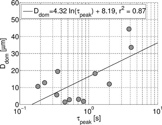
Dominant pore-throat diameters from mercury injection versus characteristic times of the IP spectra with logarithmic fit.
For increasing temperature, a decrease of the characteristic times was found for all samples that showed a peak in the measured phase spectra, agreeing with the results of Binley et al. (2010) and Zisser et al. (2010a). However, the strength of the temperature dependence varies for different samples. In order to quantify the temperature dependencies of the different characteristic times, they were fitted using eq. (6). The exponents ατ range from 0.52 to 1.42, which clearly exceeds the range from 0.8 to 0.97 reported in Zisser et al. (2010a). The equation that was used for fitting the temperature dependence of the characteristic times (eq. 6) is based on the assumption that the only temperature-dependent parameter is the ion mobility. Zisser et al. (2010a) assumed, that the ion mobility in the Stern and diffuse layers are similar to the mobility in the free electrolyte, valid for clay-free sandstones. Our results with Walden exponents different from that of the free electrolyte (αμ = 0.905), suggest that this assumption is not valid for most of the samples of this study. However, we could not find a direct relation to the clay content or other petrophysical parameters.
5.2 Comparison of theoretical and experimental results
Although we are able to fit the temperature dependence of the characteristic time of the model to that of a sandstone sample with realistic pore lengths (Fig. 9), the following considerations are not intended to demonstrate that the model exactly describes all mechanisms taking place in the pores of a sandstone. The model represents a strong simplification of the pore geometry of a sandstone and might therefore underestimate or neglect the influence of several contributing factors. However, a qualitative comparison of the temperature dependence of the IP spectra with the model can help to assess whether the theory describes relevant processes, and possibly help to understand the processes at the pore scale underlying the observed temperature dependencies.
The effective conductivity of the model (Fig. 7) is about one order of magnitude smaller than the measured conductivity (Fig. 3). This discrepancy is small considering the simple model geometry compared to the complex network of different-sized pores in series and parallel of a natural rock. Comparing the temperature dependence of the real part of the measured conductivity and the effective model conductivity, respectively, gives a qualitative agreement in the increasing behaviour for both quantities, but a strong difference of the Walden exponent with ασ(measurements) = 0.85–1.13 and ασ(model) = 2.19. Although the Walden exponent of the model is only valid for one pore size and can change when the pore size is changed, exponents similar to the ones measured only occur when both pore radii are larger than 1 μm. At large pore radii (ri ≫ λD), the EDL covers a negligible part of the pore cross section. Therefore, bulk conductivity controls the absolute value of the admittance and the temperature dependence only stems from ion mobilities and diffusion coefficients (Walden exponent αμ = 0.91). At much smaller pore radii (≪0.1 μm), as used in this study to produce sufficiently large phase shifts, the EDL covers a considerable part of the pore cross-section and the temperature dependence of the total current through the pore system also depends on the properties of the EDL. In particular, the Zeta potential increases rapidly with temperature and leads to a much stronger temperature dependence (ασ = 2.19) of the absolute value of the admittance than predicted by the modified Walden product. The difference in the Walden exponents between theoretical and measured values might imply that the model in its present form tends to overestimate the influence of narrow pores.
In the following we focus on the phase shift. The most prominent similarities of the measurements and the model are (1) the shift of the phase maximum to higher frequencies (which is equivalent to a decrease of the characteristic time) with increasing temperature and (2) different positions of the absolute maximum on the frequency and temperature axis for different samples (measurements) or pore geometries (model). These two aspects are discussed in more detail below.
5.2.1 Characteristic time
A detailed discussion of the increase of the modeled characteristic time (decrease of the peak frequency) with the pore length can be found in Bücker & Hördt (2013b). As the polarization process is mainly controlled by diffusion, the characteristic time is proportional to the square of the characteristic length of the system; τ ∝ L2, with L being the total pore length.
Figs 5 and 9 show that both the characteristic times of the model and those of the sandstone samples decrease with temperature. The fitted exponent (eq. 6) of ατ = 1.07 for the characteristic times of the model lies within the range of 0.52–1.42 of the exponents fitted to the characteristic times of the sandstone samples. It is slightly higher than the Walden exponent used for the calculation of the temperature dependence of the ion mobility (αμ = 0.91). This means, that also for the characteristic time, the temperature dependence of the model is not only controlled by ion mobility and diffusion coefficient, but also by the properties of the EDL.
5.2.2 Influence of pore geometry
The membrane polarization model predicts a strong temperature dependence of the magnitude of the maximum phase shift, which is related to polarizability. From eq. (12), it is evident that the polarizability (and thus the maximum phase shift) depends on a complex combination of the geometrical model parameters (pore lengths and radii) and the properties of the EDL. Earlier studies (Bücker & Hördt 2013b) revealed that the polarization magnitude adopts a maximum for certain combinations of pore radii r1 and r2 depending on the properties of the EDL. Our modelling results show that the temperature, at which the phase shift reaches a maximum, strongly depends on pore radii (Fig. 10). Apparently, at the temperature of maximum phase shift, the combination of Zeta potential and Debye length maximizes the polarizability for a certain geometry (predominantly pore radii). When the pore radii increase, the fraction of the EDL in the cross-section of the pore becomes smaller and the influence of the EDL decreases. Presumably, this decrease is compensated by a higher magnitude of the Zeta potential, that is reached at a higher temperature, shifting the absolute maximum to a higher temperature.
The measurements of samples TU-B1, P8 and S3 are also consistent with our modelling results, when taking into account the pore structure as observed from the CT images. The measured phase shifts of samples TU-B1 and S3 show an absolute maximum at approximately 20 and 35 °C, respectively. The phase shift of sample P8 has its maximum at a lower temperature compared to TU-B1 and S3 (Fig. 4). Actually, pores and pore throats of sample TU-B1 are narrower than those of sample S3 and wider than those of sample P8, which is in agreement with the prediction of the model. However, this observation does not hold for some of the samples, when only the dominant pore-throat radius is considered, for example, sample TU-B4 with small rdom but a maximum at 40 °C.
Another observation when comparing simulated and measured spectra is the different width of the phase peak, which arises from the pore-size distribution. The model considers only two pore lengths (and two radii), which result in a superposition of two characteristic times and corresponding phase peaks. However, Bücker & Hördt (2013b) point out, that generally only one of the pores dominates the relaxation process, which gives rise to a very narrow phase peak with steep slopes. In natural rock samples, on the other hand, a wide range of pore lengths may exist resulting in a distribution of characteristic times and a broadened phase peak. Similarly, the wide range of different pore radii in natural rock samples is supposed to cause a broad maximum of the phase shift in the temperature domain, leading to a weaker temperature dependence of the measured phase shift compared to the modeled one.
5.2.3 Properties of the model
The parameter sets used here to produce results comparable to the measured data include ratios between pore lengths and pore radii of up to 500. This seems relatively large, considering that typical pore-throat sizes of sandstone determined by mercury injection measurements are only about 1/10 of the mean grain size (e.g. Binley et al.2005; Nelson 2009). The mean grain size, in turn, is a suitable approximation for the mean pore length. The ratio 1/10 is also in agreement with the grain and pore sizes observed in the CT images of our sandstone samples.
The CT images give an idea about characteristic length scales, but they do not include information on the possible existence of submicron pores due to the resolution of approximately 1 μm. The pore radii required for calculating a phase shift similar to measured phase shifts are smaller than mean pore radii of rock samples. This discrepancy could be attributed to an underestimation of polarization effects in large pores by the model, but it is also possible that only very small pores are responsible for the polarization effect. The existence of submicron pores in our samples has been observed by the mercury injection measurements, although in most samples the dominant pore-throat diameter is larger. Also other authors have reported submicron pores for sandstone samples (e.g. Bloomfield et al.2001; Kruschwitz et al.2010). Anyway, at this stage we cannot say whether these submicron pores are relevant to the overall polarization response of our samples or not.
The model response is calculated with the assumption that the mobility in the Stern layer is equal to the mobility of the ions in the free electrolyte. This assumption is used for clean sands in several publications (e.g. Leroy et al.2008; Revil & Florsch 2010), but it might be different in the presence of clays. For example, Revil (2013) calculate a considerably smaller ion mobility of μS = 1.5× 10|$^-10 \frac{m^2}{Vs}$| for the Stern layer of clayey sandstones. In the membrane polarization model, an ion mobility in the Stern layer much lower than in the diffuse layer leads to |$\widetilde{b}_p \approx \overline{b}_p$| (see Appendix B). This means that the Stern layer does not contribute significantly to the overall conduction, if the mobility in the Stern layer is much lower than in the bulk electrolyte and the diffuse layer, which contradicts our previous idea that surface conductivity might play an important role for the temperature dependence for samples with clay content.
We conclude that the interplay between Zeta potential, partition coefficient and Stern layer mobility may not be fully understood and that further work might lead to future modifications of the model. For example, the consideration of surface conductance through the partition coefficient might not consider relevant conduction mechanisms, such as the proton hopping or Grotthuss mechanism suggested by Skold et al. (2011). Although the pore geometry might not include all characteristics of the material, that are relevant for the temperature dependence, as, for example, the material composition, the comparison of modelling results and experimental findings with regard to the pore size provides a good qualitative agreement in various respects. However, the model includes many parameters and we have not yet fully exploited the entire parameter space.
5.3 Consequences for practical applications
6 CONCLUSIONS
The investigated samples show a clear temperature dependence of the SIP response, which is apparent both in the real and imaginary part of the conductivity. The absolute maximum of the phase shift appears at different temperatures, depending on the samples. The characteristic time scales decrease with increasing temperature, displaying different strengths of the temperature dependence (Walden exponents) of different samples. This observation is in good agreement with the decrease with increasing temperature, that is predicted by previous publications. The comparison with CT images indicates that differences in the Walden exponents are related to the pore space geometry. However, we did not quantify robust quantitative relationships with measurable parameters, such as dominant pore-throat diameter or clay content. If we assume that at least ‘part of the polarization is caused by an interaction of different pore radii, a correlation with a single parameter characterizing the pore space cannot necessarily be expected.
Furthermore, we simulated the temperature dependence with a membrane polarization model that is based on a sequence of wide and narrow pores. Considering the simplicity of the model geometry, the simulated spectra reproduce several features of the measured data remarkably well. Characteristic times decrease with increasing temperature and the position of the phase maximum is affected by the pore geometry. While the mean pore length mainly controls the spectral position of the maximum phase, the pore radius (or width) determines the temperature, at which the absolute phase maximum occurs. The decrease of the modeled amplitude of the admittance and the characteristic time is stronger than the predicted decrease resulting from ion mobility only. This indicates that, additionally to ion mobility, also other temperature-dependent parameters of the EDL, such as Debye length and Zeta potential, are important.
This work was funded by Baker Hughes and the Ministry of Science and Culture of Lower Saxony, Germany, within the Geothermal Energy and High-Performance Drilling (gebo) research association. We give our thanks to the Helmholtz Centre Potsdam GFZ, namely Inga Moeck, Nicole Pastrik, Sonja Martens and Ben Norden, and Dorothea Reyer for supplying the samples. We also thank Daniel Albrecht and Manfred Stövesand for cutting the samples and Annett Zimathies for the mercury intrusion measurements.
REFERENCES
