


Summary
We present a method for imaging quasi-vertically dipping faults with surface records of reflected P waves from small earthquakes. Faults are boundaries between geological structures, such as tectonic plates, and are located in earthquake active regions such as Parkfield, California. The high degree of seismic activity enables the use of multiple seismic recordings in our fault identification algorithm. Major challenges occur because of the quasi-vertical orientation of the fault and the fact that the wave reflected by the fault and recorded by the surface receivers is not well modelled by the direct arrival of the propagating wave generated by the earthquake source. Our method uses the 2-D acoustic wave equation as the model for P-wave propagation. We assume that an approximate wave speed map on the reflection side of the fault is available and the source locations are known, for example, from traveltime tomography. We also assume that the source time function is known. The new features of our method arise because earthquake sources are located very close to the fault. This has two implications: (1) the direct arrival and the reflected wave arrive almost simultaneously, so that it is impossible to separate them on a seismogram using standard techniques, and (2) most of the reflections occur above the critical angle which introduces a distortion in the reflected wave. To overcome these difficulties we use a modelled incident wave to (1) remove the direct arrival from the data, and (2) remove the post-critical distortion from the reflected wave. We justify the distortion removal using the leading-order term of an asymptotic expansion, and an optimization procedure. To complete our algorithm we utilize some features of reverse time migration: (1) the use of full acoustic wave equation for modelling and backpropagation, and (2) zero-lag correlation of the backpropagated time reversed reflected and incident fields. We present numerical examples of fault reconstructions with synthetic data.
1 Introduction
1.1 Background: imaging steeply dipping reflectors
The problem of imaging steeply dipping reflectors is of considerable interest. The applications include imaging of salt flanks in hydrocarbon exploration and imaging of vertically dipping geological faults in the areas of high seismic activity for the purpose of earthquake prediction and response modelling.
Faults often are boundaries between geological structures. One characteristic feature of major crustal faults is that they often accumulate enough offset so that the bounding crustal structures have significantly different material properties. The other characteristic is that geological faults are often associated with a high degree of seismic activity due to the movement driving the separation. This provides the opportunity to obtain seismic recordings, due to earthquakes, that can be utilized in reflection seismology algorithms. At the same time the high degree of seismic activity also drives the necessity to accurately image the region so that crustal response to earthquakes can be characterized. Later we give a review of some of the results for recovering subsurface structure.
Standard surface seismic profiles are suitable for imaging subsurface structures with shallow dips, but are not well suited to imaging steeply dipping faults (Mooney & Brocher 1987; Eberhart-Phillips et al. 1995). Layered material is readily observed in such profiles however, so vertical or steeply dipping faults may be observed as offsets in the layers. An example is the study by Feng & McEvilly (1993). In this study the San Andreas Fault (SAF) zone is observed as a break between the series of horizontal reflectors on both sides of the fault zone.
Depth migration methods with turning waves have been used by the exploration industry to image steeply dipping or overturned crustal reflectors in the subsurface, such as vertical or overturned flanks of salt domes. An example of such a method is post-stack Kirhhoff depth migration (Ratcliff et al. 1992; Albertin et al. 2002), where a certain pre-processing needs to be applied to the data to retain the refracted reflections in the stacked data. Whitmore (1983) and Baysal et al. (1984) showed that it is possible to image overturned reflectors with turning waves using reverse time migration. A number of migration methods based on one-way wave equation, capable of processing turning waves have been proposed. Claerbout (1985, pp. 272–273) proposed a modification to the post-stack phase-shift migration algorithm; this modification enables imaging overturned reflectors with two passes of a one-way wave equation. This algorithm is applied by Hale et al. (1992) to create a 3-D image of a salt dome with overhanging flanks. True amplitude modification of this method is used by Zhang et al. (2006). Other one-way wave equation methods use a combination of extrapolation in the downward and horizontal direction (e.g. Zhang & McMechan 1997; Jia & Wu 2009), one-way wavefield extrapolation in tilted coordinate systems (e.g. Higginbotham et al. 1985; Shan & Biondi 2008), and one-way wavefield extrapolation in Riemannian coordinate systems (e.g. Sava & Fomel 2005; Shragge 2006). The common idea behind all these methods is that they use turning, that is, upwardly refracted waves in areas with depth-dependent wave speed gradient to image the steeply dipping or overturned reflectors. The differences are in the choice of migration method, and the method to extrapolate the incident and reflected wavefields if a one-way wave equation migration method is chosen.
Prestack Kirchhoff depth migration of turning waves has been applied to imaging of steeply dipping reflectors in active fault zones. Louie et al. (1988) applied pre-stack Kirchhoff migration with refracted reflections to the data collected in the Parkfield area of the SAF by the Consortium for Continental Reflection Profiling (COCORP) survey in 1977. They located and interpreted several dipping reflectors on both sides of the SAF trace, however they did not succeed in locating the vertical SAF surface. In another study by Louie & Qin (1991) this method was used to image the east branch of the Garlock Fault in California, dipping at 45°.
Hole et al. (2001) used Kirchhoff pre-stack depth migration on the data acquired in a 2-D survey, dubbed PSINE (Parkfield Seismic Imaging Ninety-Eight), which consisted of a ∼5 km line across the SAF trace. They imaged reflectors in the Parkfield area of the SAF to within about 1 km depth. They located a reflector dipping southwest from the surface trace of SAF and a reflector extending down from approximately 500 m below sea level directly beneath the trace of the Gold Hill Fault. Bleibinhaus et al. (2001) used Kirchhoff pre-stack depth migration to image steeply dipping reflectors in the subsurface up to 6 km in depth, and horizontal to moderately dipping reflectors in the deep subsurface (≈8–25 km), using the data from a 46-km-long active survey line extending across the SAF trace.
Another study that used Kirchhoff migration with data from both passive and active sources has been accomplished by Chavarria et al. (2003) to image reflectors in the SAF area near Parkfield. These authors migrated the secondary signals that appeared between the P- and S-wave arrivals, and also after the S-wave arrivals. They interpreted these signals as P-P, S-S and P-S conversions in the seismograms recorded by geophones installed in the SAFOD pilot borehole. In their work seismograms from earthquakes and calibration shots located within 8 km of the borehole were used. They located a steeply dipping reflector just below the SAF trace, as well as a dipping reflector that they interpreted to be the fault known to intersect the SAFOD pilot hole, and two other reflectors on the southwest side of the fault.
Migration is typically performed with active source data recorded at the surface or in boreholes. Migration with turning waves often requires large offsets between the source–receiver pairs and the reflector, especially when the depth-dependent wave speed gradient is not very large. This is often the case with crystalline basement rocks such as the Salinian granite and Franciscan rocks on the two sides of the SAF (Stradtlander & Brown 1997). Therefore the depth to which the methods based on turning waves can penetrate is limited by the wave speed gradient and the offset.
For vertical faults, fault zone head waves can provide a simple high-resolution tool to image the wave speed contrast across the fault surface (Lewis et al. 2007; Zhao et al. 2010).
With this review as background we now describe the setting that drives the work reported in this paper. In the areas of major faulting, for example, in the Parkfield area of the SAF, records of local microearthquakes are abundant. The presence of a sharp material property contrast across most active faults makes imaging with reflections of body waves propagating from earthquake sources a natural choice. Development of traveltime methods in recent years that can invert simultaneously for the wave speed model and the hypocentre locations (Thurber & Rabinovitz 2000), as well as methods to obtain the source time function from the data (e.g. Pratt 1999; Roecker et al. 2010), makes it possible to image the fault location using seismic recordings from earthquake, that is, passive source data.
1.2 Introduction to our method for imaging with earthquake sources
The main new feature of the method proposed in this paper is that the earthquake sources are mostly located very close to the fault surface. The implications are the following: (1) the direct and reflected waves arrive almost simultaneously at the receivers, and they are not well separated, and (2) most of the reflected waves are reflected above the critical angle. Post-critically reflected waves undergo a frequency-dependent phase shift, which demonstrates itself in the time-dependent signal as a distortion in the waveform. This phenomenon is well studied for the cases of plane and spherical waves (e.g. Brekhovskikh 1960; Pujol 2003; Aki & Richards 2009). The distorted reflected signal does not correlate well with the incident signal. Our numerical experiments with synthetic data show that when the reflected data are not corrected to remove the post-critical phase shift in our method, the reconstructed fault appears shifted into the low wave speed region with respect to the true fault location. This discrepancy increases with the increase in the incidence angle.
The problem of post-critical incidence arises in at least two other seismic imaging applications, where wide angle reflection data are used: (1) shallow overburden-bedrock interface imaging, where wide angle surveys are often done to reduce the noise in the data, and (2) cross-well exploration. Pullan & Hunter (1985) investigated the effect of the post-critical incidence on the amplitude and phase of the reflected signal in the context of the ‘optimum window reflection’ technique (Hunter et al. 1984) for shallow overburden–bedrock interface imaging. They used synthetic seismograms computed in various two-layer media, and field seismograms collected in Winkler, Manitoba, to show that the waveform of the reflected wave can undergo a significant distortion when reflected at angles above the critical. Byun & Rector (1999) investigated the effects of post-critical reflection in cross-well imaging. They found that uncorrected post-critical reflections led to cancellations of reflected signal during stacking and degraded the quality of stacked data. To the best of our knowledge no systematic theory-based methods have been proposed to correct for the waveform distortion in the post-critically reflected data.

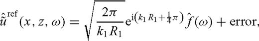
Our post-critical phase-shift removal algorithm is based on high-frequency asymptotic forms of the incident and reflected acoustic waves from a point source in two dimensions. To derive such approximations, the problem of reflection of circular waves from a planar interface in a piecewise homogeneous medium is considered theoretically. For the incident wave in such a medium the asymptotic form is well known. For the reflected wave the asymptotic form is derived from its integral representation in terms of plane waves. The accuracy of the phase-shift correction computed by our algorithm depends on the accuracy of the approximations of the incident and reflected waves by their asymptotic forms. To assess the latter accuracy, quantitative bounds on the remaining terms in the asymptotic expansions have been established.
Our method uses a few features of reverse time migration. Namely, we backpropagate the time-reversed records of the reflected wave recorded at the receivers on the surface of the earth, into a background medium, using the full acoustic wave equation. While here we demonstrate our method with synthetic data, the long-range goal is for the background medium to be constructed from the available wave speed models of the region of interest. The second similarity is the use of the zero-lag correlation with the incident field. We compute the incident field also in the background medium and backpropagate it from virtual receivers on the opposite side of the fault. The third common feature is the stacking of the zero-lag correlations from several sources.
The remainder of the paper is organized as follows. In Section 2 we describe our imaging method: removal of the direct arrival (">Section 2.1); theoretical results necessary for the post-critical phase-shift removal (">Section 2.2); our algorithm to remove the phase shift from the reflected data (">Section 2.3); and the details of our imaging method (">Section 2.4). Section 3 contains the details of our forward modelling numerical method. Section 4 contains numerical examples.
2 Outline of the fault imaging method when reflections can occur above the critical angle
The set up for the fault reconstruction problem is shown in Fig. 1. c1, ρ1, c2 and ρ2 are slowly varying wave speed and density profiles on the two sides of the fault. It is assumed that earthquakes primarily occur on the side of the fault where the wave speed is lower, which we denote c1, that is in general c1 < c2. We also assume that density is correlated with the wave speed, that is, ρ1≤ρ2. The recorded data are acoustic pressure at the surface.
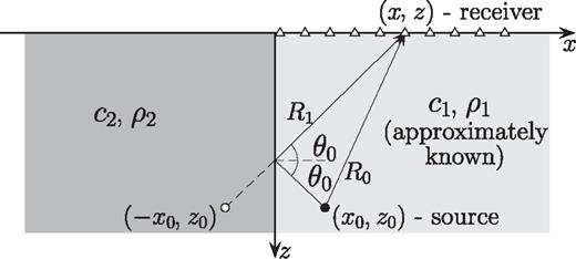
Piecewise homogeneous true medium with straight vertical fault; receivers located on the reflection side of the fault are marked by Δ. R0 and R1 are the distances travelled by the incident and reflected waves, and θ0 is the angle of specular reflection.
We assume that the following data are available for our problem: (1) an approximate wave speed model on the slower side of the fault, obtained, for example, from traveltime tomography, (2) approximate hypocentre locations, (3) an approximate source wavelet for each hypocentre and (4) the fault trace on the surface. From the surface trace of the fault we identify the receivers on the reflection side of the fault.
2.1 Removal of the direct arrival on the reflection side of the fault
We illustrate removal of the direct arrival from the total recorded wave on the medium shown in Fig. 1. The recorded data u(x, z, t) contain both the direct arrival and the reflected wave on the reflection side of the fault.

To illustrate the need for the subtraction of the incident wave, Figs 2(a)–(c) show examples of the modelled recorded signal on the reflection side of the fault, the corresponding direct arrival and the reflected wave obtained by subtraction of the direct arrival from the recorded signal, for the true medium shown in Fig. 1. In this calculation c1= 4 kms-’1, c2= 6 kms-’1 and ρ= constant. The source is located in the low speed medium 0.11 km from the fault, at the depth 4.1 km below the surface; the receiver is located at the surface, 0.6 km from the fault. The source wavelet is the Ricker wavelet with peak frequency 9 Hz. The critical angle of reflection in this calculation is 0.72973 ≈ 0.23π. The specular angle of reflection is 0.44π, thus the reflection is post-critical. The reflected wave undergoes a phase shift of ≈0.8π, so that its shape is distorted.
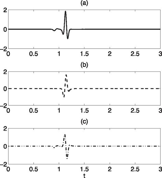
Typical time traces at receivers on the reflection side of the fault for a 2-D medium with straight vertical fault shown in Fig. 1: (a) total received signal, (b) direct arrival and (c) reflected wave. The vertical axis is amplitude.
Note that the low amplitude break with reversed polarity, which appears before time =1 s on the seismograms in Figs 2(a) and (c), is the head wave [or lateral wave in the terminology of Brekhovskikh (1960)]. It is shown in Zheglova (2010) that in the high-frequency asymptotics the amplitude of the head wave has the same order of magnitude as the error in the asymptotic representation of the reflected wave, therefore in the estimates presented in the next section the head wave is included in the error term.
2.2 Estimates needed for post-critical phase-shift removal
- (i)
 ,
,  such that c1 < c2, ρ1≤ρ2;
 - (ii)
the index of refraction, n=c1/c2 is bounded away from 0 and 1: 0 < n*≤n≤n* < 1 for some n*, n*;
- (iii)
0 ≤θ0≤π/2, i.e. all incidence angles including normal and grazing are allowed;
- (iv)
the source position is (x0, z0), where x0 > 0, z0 > 0, that is, the source is located in the slow medium;
- (v)
the receiver position is (x, z) where x > 0, z < z0, that is, the receiver is located in the slow medium above the source.
Theorem 1.
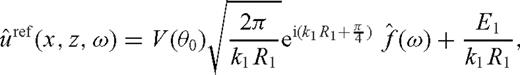
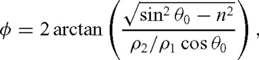
θ0 is the angle of specular reflection;  is the critical angle;
  is the distance travelled by the reflected wave;
E1 is an order 1 error term.
Theorem 2.
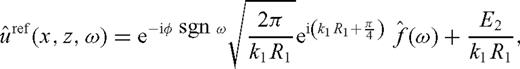
E2 is an order 1 error term.
Theorem 3.
Note that for θ0=θcr the reflection coefficient is 1.
 for large arguments. We give it here for completeness.
The results in Theorems 1–3 were obtained following the general approach employed by Aki & Richards (2009) and Brekhovskikh (1960) where similar results for 3-D spherical waves are derived.
The key features in the results above are as follows:
- (i)
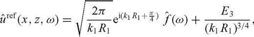
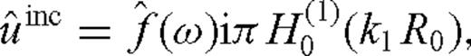
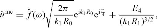
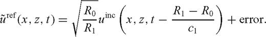
The leading terms in the above-mentioned representations of the incident and reflected waves are
 .
. - (ii)
The error term of the incident wave has the order
 .
. - (iii)
The error term of the reflected wave has the order
 when θ0≠θcr, and order
  when θ0=θcr.
 - (iv)
For θ0≠θcr the constants E1 and E2 in the error terms contain factors of the form |sin2θ0-’n2|-’1/2 and (sin(θ0-’θcr))-’1 that approach ∞ as θ0→θcr. We conjecture without proof that these factors give rise to the lower order error estimate when θ0=θcr. In other words, as θ0→θcr, the order of the error approaches
 .
.
2.3 Removal of the distortion due to reflection at angles above the critical angle
 is the Hilbert transform defined as
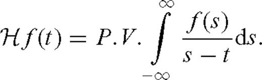
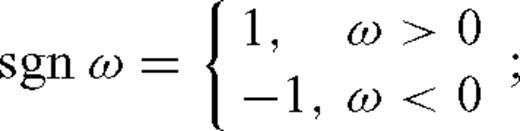
 has a frequency-dependent phase shift -’φsgnω, which translates into a distortion of the reflected waveform in the time domain as shown in (9). Our method is to make a change in
  in formula (5) at each frequency to obtain a new function
  :
: 
 to obtain the undistorted time trace
  :
: 
 and
and  to obtain
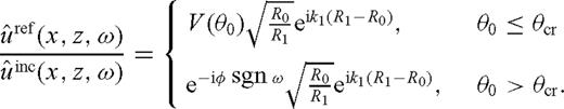
 to obtain
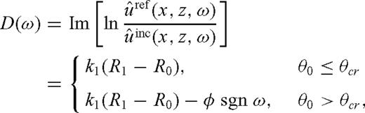
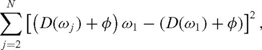
 appears in each equation, one can select φ that minimizes the following functional which is independent of
  :
: 
We use the leading-order terms of  and
and  in the derivation of formula (11) for finding φ, however in calculations with synthetic or measured data the full Fourier transform of the reflected wave uref, and the computed incident wave uinc is utilized.
2.4 The imaging method
As described earlier, our fault identification algorithm involves removal of the direct arrival from the recorded wave on the reflection side of the fault and phase correction of the reflected wave. Additionally, we note that when we compute the direct arrival we save it at locations on the transmission side of the fault. In this study we choose these virtual receiver locations to be symmetric to the receivers on the reflection side of the fault with respect to the surface fault trace. The imaging method consists of the following steps:
- (i)
Backpropagate the time-reversed phase-corrected reflected wave
 from the receivers on the reflection side of the fault in the background medium.
 - (ii)
Backpropagate the time-reversed direct arrival from the virtual receiver locations on the transmission side of the fault in the background medium.
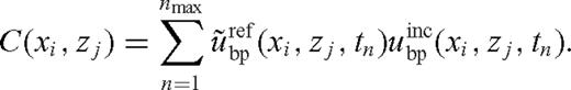
- (iii)Compute the zero-lag correlation in time of the backpropagated fields determined in steps (i) and (ii) at each point (xi, zj) of the computational domain according to the formula:12
- (iv)For each depth zj, find the range position
 where the zero-lag correlation from step (iii) is maximized: The set13
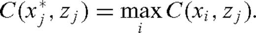
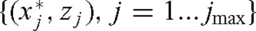 is the recovered fault location.
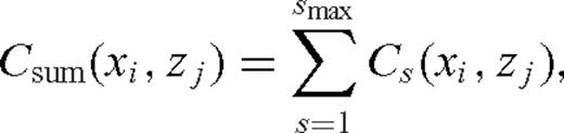
 - (v)Zero-lag correlations from several sources are summed to increase the accuracy of the reconstruction:where s is the source number. Then step (iv) is applied to Csum (xi, zj), that is, the set14
 is the recovered fault location, where 15
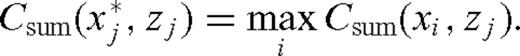
3 Forward modelling method
Calculation of the incident wave and steps (i) and (ii) of our fault imaging method require solution of the forward acoustic wave equation in the background medium; thus it needs to be solved three times for each source. In addition, to generate synthetic data we solve the forward wave propagation problem 2">(1)–(2) in the true medium.
This section describes the computational domain, the numerical scheme, our implementation of the outgoing boundary conditions, mesh parameters and interpolation procedures that we use to solve these four forward problems. We also explain our method for choosing frequencies that we use in the calculation of the phase correction φ.
To solve the above wave propagation problems, we set in all examples the density ρ to be constant throughout the computational domain. The source is modeled as the Ricker wavelet point source with the peak frequency of 9 Hz. In the case of the backpropagation problems the time-reversed records of the phase-corrected reflected/incident waves are assigned as the Dirichlet boundary conditions at the receivers/virtual receiver locations.
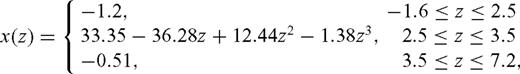
The computational domain is shown in Fig. 3. In all examples it has the following dimensions: horizontal range x=-’6.8 to x= 5 km; depth z=-’1.6 to z= 7.2 km, where z= 0 corresponds to the sea level. The surface of the Earth is assumed to be flat and is located at the depth z=-’0.6 km, that is, 600 m above sea level. Outgoing boundary conditions are applied on all sides of the computational domain, which are implemented as the Perfectly Matched Layers (PML). At the top boundary we extend the subsurface wave speed profile above the surface to the depth of -’1.6 km and impose the outgoing boundary condition at z=-’1.6.
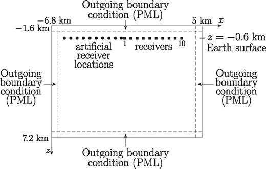
Computational domain.
To minimize the influence of using the same numerical scheme for both synthetic data generation and our inverse algorithm we use two different non-overlapping uniform meshes:
- (i)
mesh (1) is used for the synthetic data generation and has the spacing Δx=Δz= 0.020325 km; the size of the mesh is 581 × 433 grid nodes;
- (ii)
mesh (2) is used for the calculation of the incident wave and the backpropagation steps (i) and (ii) and has the spacing Δx=Δz= 0.02 km; the size of the mesh is 591 × 441 grid nodes.
The surface trace of the fault is assumed to be located at the range x=-’1.2 km in all examples. 10 receivers spaced by 500 m are placed on the surface on the reflection side of the fault between x=-’1.1 and 3.4 km. 10 virtual receivers are placed symmetrically with respect to the fault trace on the surface between x=-’1.3 and x=-’5.8 km. Both receivers and the virtual receiver locations are placed on the grid nodes of mesh (2), and the generated synthetic data computed on mesh (1) are interpolated using bilinear interpolation to obtain time traces at the receivers.
The acoustic wave equation in the interior computational domain is solved by O(Δt2, Δx10) explicit time domain finite difference scheme (Dablain 1986). The higher order scheme can significantly reduce the size of the problem, as it only requires about 3.5 samples per minimal wavelength to ensure non-dispersive propagation. In the case of synthetic data generation the wave speed has a discontinuity along the fault. We recognize that the error of the numerical solution computed with the higher order scheme can be quite high. In calculations with the background medium, the wave speed profile is smooth, so that numerical error is small. Our implementation of the PML follows the approach of Collino & Tsogka (2001) and Liu & Tau (1997). The PML are 10 gridpoints wide and occupy 10 outermost grid layers on each side of the computational domain. The order of the numerical approximation in the PML is matched to the order of the numerical approximation in the interior domain by tapering the order of spatial derivatives from O(Δx10) near the interior domain to O(Δx2) on the outside boundaries. This is necessary to minimize reflections from the boundaries between the interior domain and the PML. For the complete details of the numerical method the reader is referred to Zheglova (2010).
 Hz, for which the content is at least 10 per cent of the maximum absolute frequency content of the computed incident wave:
4 Numerical results
In this section we present numerical examples. First we present examples of fault reconstructions without noise. Then we present examples demonstrating performance of the method under uncertainty in source location and background wave speed, and in the presence of a fault zone.
4.1 Numerical results without noise
Here we present three numerical examples. In Example 1 we perform a reconstruction of a straight vertical fault separating regions of constant wave speed, as shown in Fig. 4(a). The wave speed in the low- and high-speed region is c1= 4 kms-’1 and c2= 6 kms-’1, respectively. The reconstruction is done with a single source located at (-’1.09, 3.5).
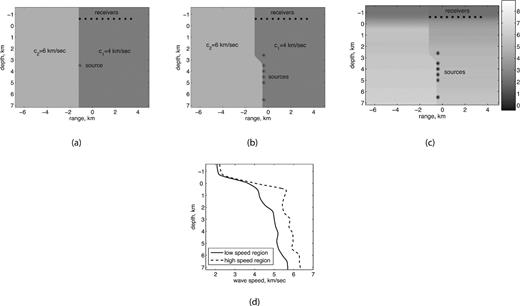
True media: (a) Example 1, (b) Example 2 and (c) Example 3. (d) Wave speed profiles in Example 3.
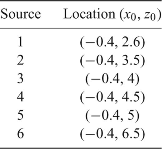
Source positions in numerical examples 2 and 3.
Fig. 5 shows the image of the zero-lag correlation and the recovered fault location for Example 1. We infer from Fig. 5 that our method can produce a very good recovery in this benchmark example with data from a single source. Since the shape of the fault is simple, it is possible to calculate theoretical value of φ predicted by geometric optics, formula (6), and compare it with the value of φ obtained in our phase-shift removal algorithm, that is, by minimizing functional (11). Table 2 shows both values of φ for each receiver. Reflections arriving at receivers 1–9 are post-critical. At receiver 10 the value φ= 0, predicted by geometric optics, corresponds to subcritical reflection. The values of φ computed by our algorithm are consistent with the values of φ predicted by geometric optics at receivers 1–5, and get progressively less accurate at receivers 6–10, where the reflection angle gets within 14° of the critical angle. This is consistent with the results of Section 2.2, where we showed that the approximation of the circular reflected wave by its leading-order term is the least accurate near the critical angle.
Example 1: (a) Image of the zero-lag correlation computed according to formula (12) described in step (iii) of our imaging method; (b) reconstruction of the fault location obtained by the procedure described in step (iv), imaging condition (13).
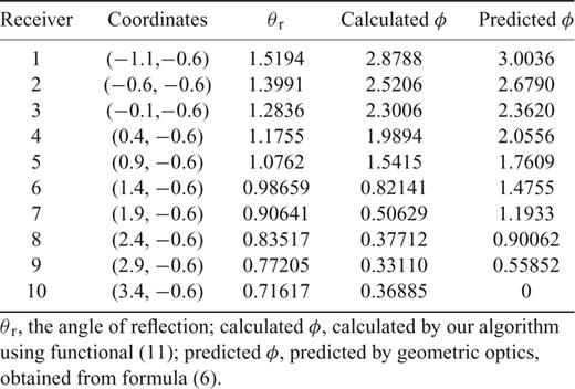
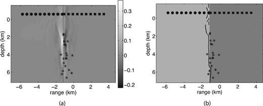
Fig. 6 shows the image of the stacked zero-lag correlations from all sources and fault reconstruction for Example 2. For comparison, Figs 7 and 8 show reconstructions with the data from single sources 1 and 5. Source 1 is shallow, therefore the upper segment of the fault is recovered very well. With the deeper source 5 the lower segment of the fault above source is recovered best. We note that a significantly better image of the whole fault is obtained from the zero-lag correlation stack (Fig. 6). We also note that we obtained a good recovery with a small number of sources.
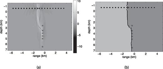
Example 2: (a) Image of the sum of the zero-lag correlations from sources 1–6 computed according to formula (14), step (v) of our imaging method; (b) reconstruction of the fault location with imaging condition (15), step (v). The source locations are given in Table 1.
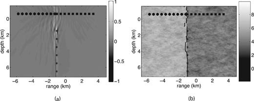
Example 2, source 1: (a) image of the zero-lag correlation computed according to formula (12), step (iii) of our method; (b) reconstruction of the fault location with the imaging condition (13), step (iv). The source location is (-’0.4, 2.6).
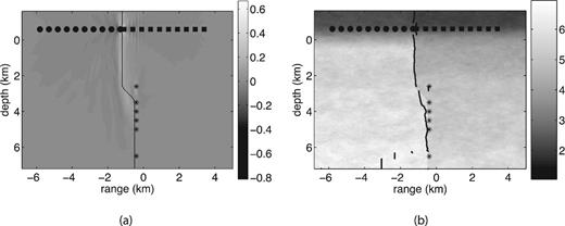
Example 2, source 5: (a) image of the zero-lag correlation computed according to formula (12), step (iii) of our method; (b) reconstruction of the fault location with the imaging condition (13), step (iv). The source location is (-’0.4, 5).
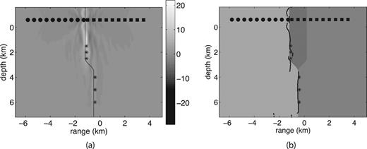
Fig. 9 shows the image of the zero-lag correlation stack and fault reconstruction for Example 3. We do not include any reconstructions of the fault with single sources for this example, but they can be found in Zheglova (2010).
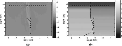
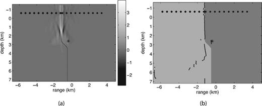
Example 3: (a) image of the sum of the zero-lag correlations from sources 1–6 computed according to formula (14), step (v) of our imaging method; (b) reconstruction of the fault location with imaging condition (15), step (v). The source locations are given in Table 1.
The straight parts of the fault in Figs 6 and 9 are imaged better than the shifting parts. In Fig. 6 the location of the shift is shown correctly and the reconstruction gives a clear indication of its shape, but it does not render correctly the incline of the shift. In Fig. 9 the shape of the shift is rendered correctly, but the steepness of the shift and its location are not reconstructed quite correctly. One reason for this is that our imaging method is naturally better suited to image straight vertical reflectors, as it takes advantage of the symmetry of the incidence and reflection angles that straight faults provide. The other reason is that reflections from non-straight interfaces can include multiply scattered waves, multiple reflected arrivals from several parts of the fault arriving at the same receiver and refractions. Our algorithm is designed to make good use of singly reflected waves but it is not well suited to take into account multiples and waves refracted across the fault. Also, our algorithm does not distinguish between several reflected arrivals and treats them all as a single reflected wave. Typically the waves that are singly reflected dominate in amplitude, so that they have dominant weight in the calculation of φ, and produce the largest values of the the zero-lag correlation. Thus the straight parts of the fault from which waves are singly reflected are imaged better.
4.2 Sensitivity of the method to uncertainty in source location
In practice exact knowledge of the earthquake source locations is not achievable. To determine sensitivity of the proposed method to errors in the source location we conducted a series of experiments where modelled incident waves from randomly perturbed sources were used to recover the fault with our method. In these tests we used the fault configuration of Fig. 4(a). We assumed 20 sources located along two straight lines at x=-’1.09 km and x=-’0.8 km. The depths of the sources ranged from 2 to 6.5 km with a spacing of 500 m. We assumed a normal distribution of the absolute source location perturbation with an SD ranging from 100 to 500 m, and a uniform distribution of the direction of perturbation. The results for SDs of 100, 300 and 500 m are shown in Figs 10–12 (the rms deviations from the true sources are, respectively, 107.3, 246.2 and 500.3 m). We found that with the current range of frequencies in the source the method produces good recoveries with SD of up to 150 m, which is about 2 per cent of the depth of the deepest source. Above this margin the method is somewhat sensitive to how many sources are actually well located. For example we obtained a good fault recovery with SD of absolute perturbation of 300 m, and a rather unacceptable recovery with SD of 500 m. We find that our method is more sensitive to perturbation when we cancel the direct arrival and we compute the phase correction φ, and less sensitive in the backpropagation step. We obtained improvements in recovery with 500 m SD by using the incident wave from exact sources to cancel direct arrivals and to compute φ (Fig. 13). This suggests that robustness of our method can be improved by increasing the number of sources, and by elimination of the modelled incident wave from the data processing steps of our method. We are currently exploring the possibility of achieving separation of the direct and the reflected arrivals and computation of φ without the use of a modelled incident wave. We will report on this in a future paper.
Straight fault recovery with perturbed sources: (a) zero-lag correlation stack; (b) reconstruction of the fault location. SD of the absolute source location perturbation is 100 m.
Straight fault recovery with perturbed sources: (a) zero-lag correlation stack; (b) reconstruction of the fault location. SD of the absolute source location perturbation is 300 m.
Straight fault recovery with perturbed sources: (a) zero-lag correlation stack; (b) reconstruction of the fault location. SD of the absolute source location perturbation is 500 m.
Straight fault recovery with perturbed sources, when exact incident wave is used for direct arrival removal and computation of φ: (a) zero-lag correlation stack; (b) reconstruction of the fault location. SD of the absolute source location perturbation is 500 m.
4.3 Sensitivity to uncertainty in model parameters
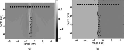
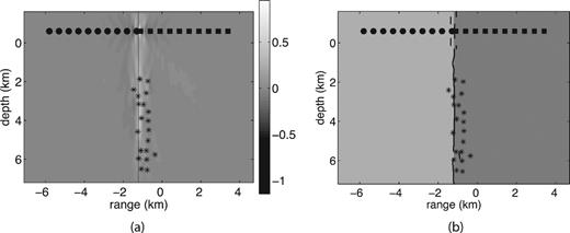
In general the wave speed model recovered by tomography methods is not precise. The minimum structure regularization that is typically used in traveltime tomography algorithms produces smooth wave speed models and the resolution depends on ray coverage. To study the sensitivity of our method to uncertainty in the background model we added random variations to the models from Figs 4(a) and (c), and reconstructed the fault using the homogeneous and depth-dependent background media of Examples 1 and 3, respectively. The variations in the true wave speed had zero mean and a von Karman covariance function of order 0.3. Characteristic lengths in the range and depth directions were chosen to be 0.4 and 0.2 km, which is 90 per cent and 45 per cent of the peak wavelength. The rms wave speed variations of 3, 5, 7 and 10 per cent of the low wave speed for the model in Fig. 4(a) were chosen, and 1 and 3 per cent of the wave speed for the model in Fig. 4(b). In all tests we obtained good fault recoveries. The results for the two media with rms variations of 10 and 3 per cent, respectively, are shown in Figs 14 and 15.
Straight fault recovery in the variable medium with rms wave speed variation of 10 per cent: (a) zero-lag correlation stack; (b) reconstruction of the fault location.
Shifting fault recovery in the variable depth-dependent medium with rms wave speed variation of 3 per cent: (a) zero-lag correlation stack; (b) reconstruction of the fault location.
4.4 The effect of the fault zone
In many cases faults represent a narrow zone of fractured or partially consolidated rocks at least at shallow depths. At deeper depths the assumption of a sharp interface is well supported by observations (Ben-Zion & Sammis 2003). The presence of a fault zone may have significant effect on our method, due to the following factors:
- (i)
if the wave speed in the fault zone differs significantly from the surrounding rock it needs to be accounted for in the background model to ensure the correct speed of the backpropagated waves;
- (ii)
in the wide angle regime most of the energy is trapped inside the fault zone, and the waves propagating outside the fault zone are evanescent and
- (iii)
the walls of the fault zone produce multiple reflections.
We conducted a series of tests where a low-velocity fault zone was introduced into the true models of Figs 4(a) and (b). We used the wave speed of 3.2 kms-’1 in the fault zone and varied its width and shape. We found that our method works well with very narrow fault zones (∼ 100 m), and with relatively wide fault zones (over 1 km wide). In the latter case the fault zone wave speed is used as the background wave speed and multiple reflections from the fault zone boundaries are muted. We note that muting is possible in this case, since multiples are well separated from the incident wave and the primary reflections. Muting the multiples is especially effective when imaging deeper parts of the fault zone. One possible reason for this is that due to wide angle incidence, the waves recorded at receivers located closest to the fault give the most contribution to the fault image for shallower depths. For deeper parts of the fault zone, the contribution from more distant receivers becomes important. The direct wave and the reflections that would travel to those receivers become trapped in the fault zone waveguide and produce multiples. These multiples, when backpropagated into a homogeneous background medium, cause artefacts on the zero-lag correlation image.
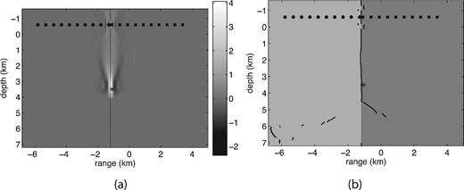
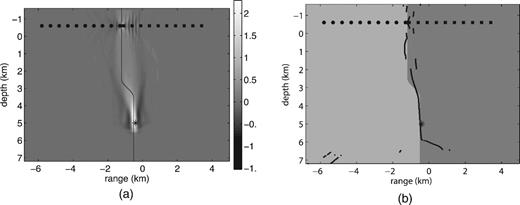
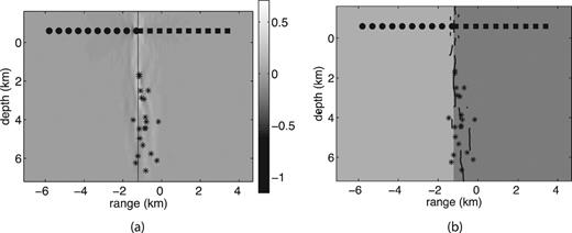
Fig. 16 shows an example of fault reconstruction in the medium that is obtained from the medium in Fig. 4(b) by adding a 1.4-km-wide fault zone that tapers to a straight line at 3.5 km depth. Three sources are placed inside the fault zone close to its left boundary at depths z= 1.5, 2 and 2.5 km and range x=-’1.09 km, and three more sources are located below the fault zone close to the fault at depths z= 4, 5 and 6 km and range x=-’0.4 km. The geometry and wave speed contrasts are chosen so that they are roughly representative of the SAF near Parkfield (Thurber et al. 1997; Catchings et al. 2002; Hole et al. 2006). The homogenous background wave speed of 3.2 kms-’1 is used to recover the fault location with the three sources located in the fault zone, and 4 kms-’1 background wave speed is used for the three deeper sources. The zero-lag correlations from the six sources are stacked. The overall features of the fault, except the horizontal shift, are well imaged.
Fault recovery in the presence of fault zone: (a) zero-lag correlation stack; (b) reconstruction of the fault location.
With fault zones of intermediate widths the quality of reconstructions varied significantly with the shape, width and depth of the fault zone, as well as the number and locations of the sources. The analysis of the fault zone scenario and proper modifications to our method will be addressed in a future study.
5 Conclusions
In this paper we proposed a method of imaging quasi-vertical geological faults with earthquake data. Our method assumes prior knowledge of an approximate source location and wave speed profile in the reflection medium, which are usually available. Our method also assumes the knowledge of the source time function.
In this paper we addressed two problems associated with wide angle reflection imaging that arise from the earthquake sources being very close to the fault surface: (1) separation of the incident and reflected arrivals, and (2) imaging with post-critically reflected waves. We provided a theoretical framework allowing construction of a systematic way to remove the post-critical phase shift from the reflected wave.
Currently our method is implemented in two dimensions and the wave propagation is assumed to be governed by the acoustic wave equation.
We tested our method on synthetic examples with noise-free data in piecewise homogeneous and depth-dependent media with two types of fault configurations. We also assessed numerically the sensitivity of our method to various kinds of noise in the data, and investigated to some degree performance of our method in the presence of a fault zone.
The questions that this study does not address and that we consider our future work directions include the following:
- 1
Elimination of the computed incident wave from the data processing steps of our method to improve robustness to uncertainty in the source location. This can be achieved by formulating the arrival separation and phase-shift correction steps as an optimization problem, where the incident and the reflected wave traveltimes and the phase correction φ are fitted to the recorded waveforms at each receiver, using our asymptotic formulae. It is a fully non-linear optimization problem with a highly oscillatory objective function, however the forward computation is fast, so that it can be handled efficiently by Bayesian inversion combined with a global optimization engine. Preliminary tests of this approach with synthetic data suggest that the problem is more sensitive to the incident arrival time than to the reflected arrival time and φ.
- 2
Development of a procedure to construct the background medium that accurately represents the true wave speed in the low-speed region from a reconstruction of the true wave speed that is not exact or too smoothed out in the vicinity of the fault, such as occurs in a traveltime tomography reconstruction.
- 3
Further investigation of our method in the presence of a fault zone.
- 4
Generalization of our method to 3-D elastic media and incorporation of the anisotropic source radiation pattern into the modelling process.
Acknowledgements
The authors, SR, PZ and JMcL were partially supported for this work by the NSF grant: DMS 037634. JMcL was partially supported by ONR: NOOO14-08-0432. J-RY was partially supported by NSF Focus Group grant: DMS 0101458. DR was partially supported by the NSF VIGRE award: DMS 9983646.
References
