


Summary
Finite-fault source inversions reveal the spatial complexity of earthquake slip or pre-stress distribution over the fault surface. The basic assumption of this study is that a stochastic model can reproduce the variability in amplitude and the long-range correlation of the spatial slip distribution. In this paper, we compute the stochastic model for the source models of four earthquakes: the 1979 Imperial Valley, the 1989 Loma Prieta, the 1994 Northridge and 1995 Hyogo-ken Nanbu (Kobe). For each earthquake (except Imperial Valley), we consider both the dip and strike slip distributions. In each case, we use a 1-D stochastic model. For the four earthquakes, we show that the average power spectra of the raw, that is, non-interpolated, data follow a power-law behaviour with scaling exponents that range from 0.78 to 1.71. For the four earthquakes, we have found that a non-Gaussian probability law, that is, the Lévy law, is better suited to reproduce the main features of the spatial variability embedded in the slip amplitude distribution, including the presence and frequency of large fluctuations. Since asperities are usually defined as regions with large slip values on the fault, the stochastic model will allow predicting and modelling the spatial distribution of the asperities over the fault surface. The values of the Lévy parameters differ from one earthquake to the other. Assuming an isotropic spatial distribution of heterogeneity for the dip and the strike slip of he Northridge earthquake, we also compute a 2-D stochastic model. The main conclusions reached in the 1-D analysis remain appropriate for the 2-D model. The results obtained for the four earthquakes suggest that some features of the slip spatial complexity are universal and can be modelled accordingly. If this is proven correct, this will imply that the spatial variability and the long-range correlation of the slip or pre-stress spatial distribution can be described with the help of five parameters: a scaling exponent controlling the spatial correlation and the four parameters of the Lévy distribution constraining the spatial variability.
1 Introduction
The source of complexity in earthquakes is not well understood and still debated (Carlson & Langer 1989; Rice 1993; Madariaga & Cochard 1994). Like other complex systems observed in nature, the expectation that the complexity of earthquakes may be due to some underlying scaling law comes from observations. The foremost observation in seismology is the Gutenberg-Richter statistics for the number and magnitude (energy release) of earthquakes (Gutenberg & Richter 1942). A less well known, but critical, observation is the roughness of topography of sliding surfaces (fig. 4 in Power 1987). Their basic result shows that over 11 orders of magnitude in fault surface wavelength—that is from field data to the laboratory—the power spectrum density of roughness (geometrical complexity) appears to follow a power law. This suggests that asperities and barrier are distributed—over a large range of scale—on the fault surface.
A faulting model of the 1979 Imperial Valley earthquake was determined by trial-and-error comparison of synthetic particle velocity with near-source recordings (Archuleta 1984). The spatial distribution of the slip was calculated on a grid with 1.0 km spacing down dip and 2.5 km along the strike. The fault surface extends from the surface to 13 km down dip and 35 km along the strike. Only the strike slip values were used in this study.
Following early observations of complexity in earthquakes (Wyss & Brune 1967; Das & Aki 1977; Aki 1979; Day 1982; Boatwright 1984), the complex behaviour of earthquakes has been reported in almost every article based on inverting near-source data for the slip or pre-stress distribution of the causative fault (e.g. Hartzell & Heaton 1986; Beroza & Spudich 1988; Bouchon 1997; Bouchon 1998a, b; Sekiguchi 2000; Zeng & Chen 2001; Mikumo 2003; Zhang 2003). In a study of spatial heterogeneity and friction in the crust, Rivera & Kanamori (2002) concluded that ‘heterogeneity of stress field, and friction in the crust seems to be the essential feature of the crust, and studies on earthquake rupture dynamics must take these heterogeneities into consideration’. As elsewhere in physical sciences, efforts to understand complex spatial variability were based on a statistical characterization approach (Boore & Joyner 1978; Andrews 1980; Von Seggen 1981; Lomnitz-Adler & Lemus-Diaz 1989; Gusev 1992; Herrero & Bernard 1994; Oglesby & Day 2002). Most of the models discussed in the literature are either phenomenological in nature or simply a guess. While these models may reproduce some qualitative features of the ‘heterogeneous’ variability observed in slip or pre-stress distribution, the model parameters are neither fixed nor validated through a comparison with the inverted slip data. Mai & Beroza (2002) went a step further and undertook such a study. Using available source models, they validated and computed the parameters of the Von Karman function that they used to model the two-point statistics of the slip distributions. Guatteri (2003), computed kinematic, hybrid and dynamic scenarios of ruptures based on synthetic random pre-stress spatial distribution modelled according to Mai & Beroza (2002). A major finding of Guatteri (2003) was that the inclusion of variability in the source parameters is fundamental to simulate realistic ground motion time series. In a paper discussing the dynamic inversion and modelling of the 1992 Landers earthquake, Peyrat (2001) concluded that rupture propagation is ‘critically determined’ by the pre-stress spatial distribution. These results suggest that proper quantification of the statistical properties associated with earthquake source models should go beyond ‘trial and error’ random modelling of the slip and pre-stress spatial heterogeneity.
In a search for a generalized model that characterizes the spatial distribution of heterogeneity over the fault surface, one has to find a model that includes and preserves as many features of the random or stochastic nature observed in the source models as possible. Gusev (1992) outlined the procedure to achieve this goal. In principle, the random model will include one-point statistics (probability law governing the distribution of the random variables), two-point statistics (correlation function or spectrum), three-point statistics and so on. Lavallée & Archuleta (2003) introduced a random model of slip distribution that was validated and parametrized by computing the one-point statistics and two-point statistics associated with the Imperial Valley source model (Archuleta 1984). The results presented in Lavallée & Archuleta (2003) depart significantly from previous studies in several aspects. First, the analysis is performed on non-interpolated data; the effect of interpolation can be profound. Second, the probability law of the random variables associated with the slip is non-Gaussian; it is a Lévy law. As shown in this paper, the usually assumed Gaussian law fails to mimic the basic results found from the data: namely a Gaussian law does not reproduce the degree of spatial variation in slip amplitude observed on the fault. As such, a Gaussian law leads to less heterogeneity in the slip and the resulting ground motion. The difference between slip heterogeneity distributed according to a Lévy law and slip heterogeneity distributed according to a Gauss law is more obvious when watching the movie of a spontaneously propagating rupture—the movie is available at .
Empirical observations of the Lévy law have been reported in seismology. For instance, analyses of the statistical properties of strong ground motion recorded in the epicentral areas of large earthquakes demonstrate that the distribution of peak acceleration is non-Gaussian (Gusev 1996). The probability density function (PDF) is characterized by ‘heavy tails’ (a typical signature of Lévy law) and is better approximated by a Cauchy law (a special case of the Lévy law) (Tumarkin & Archuleta 1997). These results suggest that observation of non-Gaussian distribution in the strong ground motion could have its origin in the spatial variability of the slip over the fault surface or vice-versa. Furthermore, Kagan (1994) and Marsan (2005) have shown that the stress increments caused by a fractal set of earthquakes on subsequent earthquakes is also distributed according to a Lévy law.
In this paper, we derive the stochastic model for the source models of four earthquakes: the 1979 Imperial Valley, the 1989 Loma Prieta, the 1994 Northridge and 1995 Hyogo-ken Nanbu (Kobe). For each inversion model (except Imperial Valley), we consider both the dip and strike slip distributions. In each case, we use a 1-D stochastic model. This choice is not the result of any particular insight or theoretical motivation but is based on pragmatic considerations. Usually source models have a larger spatial extension along the strike direction than along the dip direction. The number of events (or subfaults) is then larger in the former case, often constraining the statistical analysis to layers along this direction. Fortunately, the Northridge inversion is a welcome exception to this rule, and for this purpose, it is also analysed but assuming a 2-D stochastic model. Finally in the appendix, we discuss the procedure used to compute the parameters of the Lévy law.
2 Stochastic Model of Earthquake Slip Spatial Distribution: Overview
In Lavallée & Archuleta (2003), we proposed and tested a model that includes one-point and two-point statistics for the slip distribution of 1979 Imperial Valley earthquake. The stochastic model is similar to the fractional Brownian motion (fBm)—see Peitgen & Saupe (1988), and Falconer (1990). One of the procedures used to obtain fBm, consists in generating white noise that is distributed according to a Gaussian law over a grid or lattice (of any number of dimensions), and then filtering the noise in the Fourier space to generate a ‘stochastic or random process’ characterized by a spectrum with a power-law behaviour. In Lavallée & Archuleta (2003), we relaxed the constraint that the random variables had to be distributed according to a Gaussian law and assumed the most general case of the Lévy, or stable law, (Feller 1971; Grigoriu 1995; Nikias & Shao 1995; Uchaikin & Zolotarev 1999; Sornette 2004). The underlying idea in adopting this generalization of fBm is that the probability laws, as well as the PDF parameters characterizing the stochastic model, are both fixed by the data. As we will see in the next sections, assuming that the one-point statistics are best described by a Gauss law is too restrictive and not very accurate (see also Lavallé & Archuleta 2003, 2005; Lavallée & Beltrami 2004).
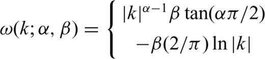
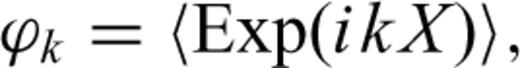
The Lévy law (also denoted the stable law, Lévy-stable law or the α-stable law in the literature) is the most general law for which the Central Limit Theorem applies—specifically the sum of (independent and identically distributed—iid) Lévy random variables is also distributed according to a Lévy law. The Lévy law is characterized by four parameters α, β, γ and μ. The parameter α, with 0 < α≤ 2, controls the rate of falloff of the tails of the PDF. The larger the value of α, the less likely it is to find a random variable far from the PDF maximum. The case α= 2 corresponds to the Gaussian law; the case α= 1 with β= 0 corresponds to the Cauchy law. The parameter β, with −1 ≤β≤ 1, controls the departure from symmetry of the PDF curve. When β= 0, the PDF is symmetric. The parameter γ, γ > 0, is mainly responsible for the PDF width. When α= 2, the parameter γ is related to the variance σ2 of the Gaussian law by γ=σ2/2. The parameter μ is the location or shift parameter. When α= 2, then μ corresponds to the mean value, and when α= 1 (with β= 0) it corresponds to the location parameter of the Cauchy law. (See also the Appendix for additional details).
The basic difference between a Gaussian law and a Lévy law can be illustrated by comparing the distribution of heights with the distribution of annual incomes for American adult males (Montroll & Shlesinger 1983). An average individual who seeks someone twice or three times his height would likely fail. On the other hand, it would not be difficult to find a person with twice or three time one's income. Systems at equilibrium or near the equilibrium are often devoid of large fluctuation—this is the reason why they remain at equilibrium—and can be (although not necessarily) described by the Gaussian law. However, non-equilibrium system are characterized by large fluctuations that can be best accounted by a Lévy law. It should not be a surprise that earthquake slip or pre-stress belongs to the latter because the slip is inferred from ground motion recordings following an earthquake—a truly non-equilibrium phenomenon.
There are three assumptions made in the application of this stochastic model to experimental data. First, we assume that the Lévy PDF are truncated, indicating that random variables are bounded between minimum and maximum values. However, we also assume that these values are large enough so that the Central Limit Theorem still applies (see Paul & Baschnagel 1999 and references therein for a discussion on the validity of the Central Limit Theorem for truncated Lévy random variables; for an interesting discussion of the ‘unbounded’ nature of probability law such as the Lévy law see the Introduction in Nikias & Shao 1995 or Sornette 2004).
A common feature exhibited by ‘complex data’ in seismology (or related disciplines) is the presence of scaling laws. Accurate computation of such scaling laws and the range of their validity are still open to debate. The second hypothesis adopted in this study, is that the scaling law can only be observed and computed on average. The scaling law does not have to be observed locally, that is, at a particular location, over a set of subfaults or layers of the slip spatial distribution. Local deviations from the scaling law are expected for a finite—or small enough number—of events. Borrowing from the terminology and conceptualization used in statistical physics, we assume that the scaling law is ‘canonical’, that is, that it can be only properly observed and computed when averaged over many events. In a canonical description of the statistical properties of a system, the average energy is conserved, while in a microcanonical description the energy is exactly preserved everywhere in the system. Note also that this requirement is rather typical for processes described by fBm or similar random processes. The concept of canonical and microcanonical descriptions have also been discussed in the context of another stochastic model called cascade processes (for instance see Lavallée 1991).
In Andrews (1980), the scaling behaviour of the slip (or pre-stress) spatial distribution was based on the assumption that the seismic process is scale independent in a broad band region delimited by the characteristic length scale of the brittle seismogenic region (∼104 m) and the grain size of the medium (∼10−2 m). Thus, a more accurate formulation of the scaling law associated with the spectrum of the slip will restrict the power-law behaviour to a finite subrange of the wavenumber k values. This subrange can be defined as the scaling subrange extending from a minimum wavenumber kmin∼ 10−4 m−1 to a maximum kmax∼ 102 m−1. Between these two limits, we assume that the slip can be approximated by the stochastic model discussed above. This is the third hypothesis adopted in this study. It is similar to the formulation of the Kolmogorov law for turbulent flow velocity, which is only observed within the ‘inertial subrange of wavelength’ (see Monin & Yaglom 1987; McComb 1991; Frisch 1995, for additional details).
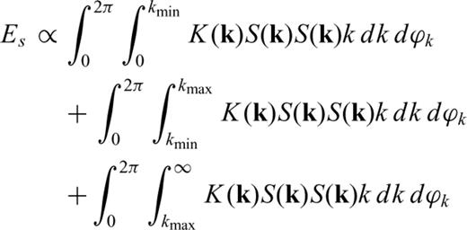
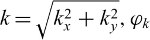 the azimuthal angle in the k domain, and K(k) the static stiffness function. The integration over k is divided in three regions, k < kmin, kmin≤k≤kmax, and k > kmax, with kmin and kmax corresponding, respectively, to the upper and lower bounds delimiting the scaling subrange. The third hypothesis adopted in this study stipulates that S(k) scales with a power-law behaviour when k satisfies kmin≤k≤kmax. Thus there is no divergence of the second integral on the left hand side of eq. (1) as long as kmin and kmax have finite and non-zero values. There is no divergence of the first and third integrals in eq. (1) assuming that the functions S(k) and K(k) are such that the product K(k)S(k)S(k)k decreases fast enough as k→∞ (see Appendix A2 and A3 in Mai & Beroza 2002) and is not singular as k→ 0. Herrero & Bernard (1994) reached a similar conclusion regarding the computation of the rms value of the stress drop obtained by integrating the stress drop over a finite range of wavenumber values. That is, the integration in eq. (1) cannot be used to constrain the value of the scaling exponent of the 2-D stress drop power spectrum.
Finally, we also assume a linear relationship between the pre-stress and the slip spatial distributions (Andrews 1980). Thus, the pre-stress and the slip spatial distributions have similar random properties that can be also related by linear relationships.
3 1-D Stochastic Model
3.1 Formulation of the stochastic model
3.2 Stochastic modelling of earthquake source models
In this section, we discuss the computation of the parameters of the stochastic model for the dip and strike slips for four earthquakes. There are several features that distinguish our computation from the stochastic modelling discussed in Somerville (1999) or Mai & Beroza (2002). First in both of their studies, the slip data were interpolated before performing the Fourier analysis. The interpolation creates additional correlations in the data and leads to a spurious estimation of the scaling exponent (for discussion and illustration see Lavallée & Archuleta 2003, and Section 4.2). The second difference is a consequence of the interpolation schemes used by Somerville (1999) or Mai & Beroza (2002): in both papers, the Fourier analysis is performed in 2-D, a luxury that one does not have when sticking to the original slip distribution (except for the Northridge source model that will be considered in the next section). A third difference is that they considered the vector sum of the slip amplitude while we use both the dip and strike slip amplitudes separately. There is no fundamental reason motivating our choice. However, analysis of the slip along the dip and strike provides more data to analyse and to validate the stochastic model. This procedure allows comparing how the parameters of the stochastic model vary with the slip direction. (For the 1979 Imperial Valley earthquake, we only considered the strike slip because there is almost no spatial variability in the inverted dip computed by Archuleta 1984.)
The dip and strike slip spatial distributions of the 1989 Loma Prieta, the 1994 Northridge and 1995 Hyogo-ken Nanbu (Kobe) earthquakes (see Figs 1–3), as well as the strike slip of the 1979 Imperial Valley earthquake (Fig. 4), are analysed according to the following procedure.
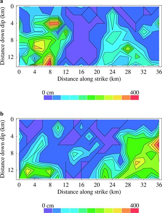
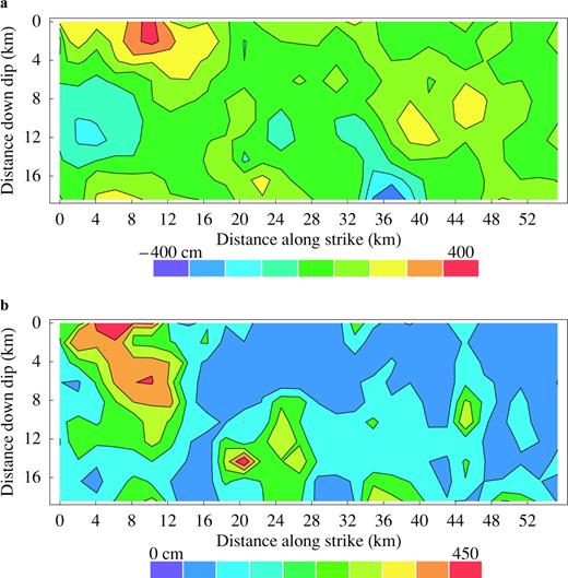
The fault slip of the 1989 Loma Prieta earthquake obtained by inverting strong motion velocity time series (Steidl 1991). The slip used in our paper corresponds to model 14 discussed in Steidl (1991). The spatial distribution of the slip was calculated at every 2 km along both the downdip and the strike directions of the fault surface. The spatial variability of the dip slip (a) and the strike slip (b) are illustrated as coloured contours on the fault plane.
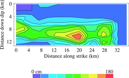
The slip distribution of the 1994 Northridge earthquake is based on the inversion of strong ground motion data (Liu and Archuleta 2000, and 2004). The slip was calculated every 1.7 km along the downdip direction of the fault surface that extends over 24 km, and every 1.76 km along the strike that extends over 20 km. The spatial distributions of the dip slip (a) and strike slip (b) are contoured onto the fault.
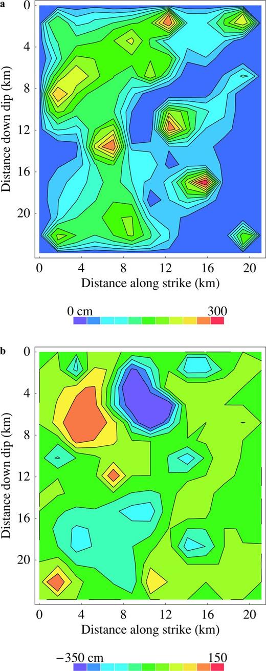
Slip distribution of the 1995 Hyogo-ken Nanbu (Kobe) earthquake based on strong motion records (Sekiguchi 2002). The fault plane is divided in subfaults located at 2.05 km intervals in both the strike and the dip directions. The spatial distributions of the dip-slip (a) and strike-slip (b) are mapped onto the fault.
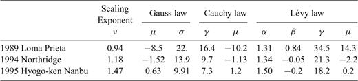
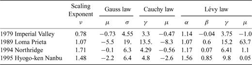
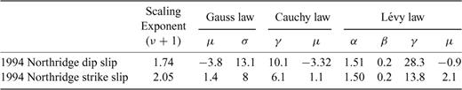
For each distribution, we computed the mean power spectrum P(kx) by dividing the slip distribution into equally spaced horizontal layers; for each layer we computed the power spectrum and then averaged over all layers—see Figs 5(a) and (b). For each distribution, the spectrum shows that there are no dominating wavenumbers, which suggest that the data cannot be reduced to—or understood as—a combination of several periodical functions. The curves show that all the wavenumbers contribute to the slip variability, and that the weight of the wavenumbers approximately follows a trend given by a decaying power law (see eq. 3). The values of the scaling exponents ν are reported in Tables 1 and 2 for the dip and the strike slip distributions, respectively. Note that assuming that these results can be extended to an isotropic 2-D stochastic model, then the 2-D power spectrum density will have a power-law behaviour characterized by a scaling exponent ν+ 1 (see Peitgen & Saupe 1988, and Section 4). According to the results given in Tables 1 and 2, the scaling exponent ν+ 1 will take values that range from 1.78 to 2.71 for the 2-D power spectrum density.
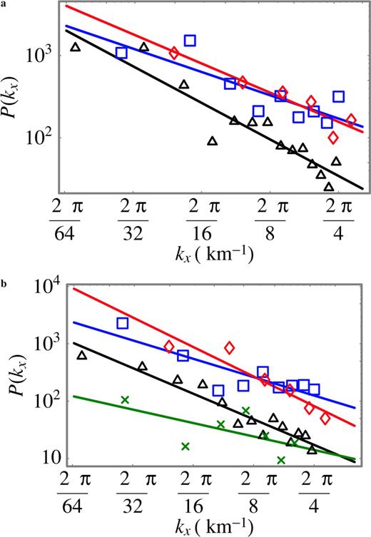
The mean power spectrum P(kx) as a function of the wavenumber kx, and the best straight line that fits the log–log curve are reported for the slip distributions of the Hyogo-ken Nanbu (black triangle ▵), the Imperial Valley (green cross ×), the Loma Prieta (blue square □) and the Northridge (red diamond ⋄) earthquakes. These results suggest that the scaling behaviour is observed for a scale length that ranges from 2 to 64 km. The values of the scaling exponent for each earthquake are given in Tables 1 and 2. The quality of the fitted curves illustrated in (a), as estimated by the values of the linear correlation coefficient (in absolute values), goes from average (0.84 for Loma Prieta) to good (0.94 for Hyogo-ken Nanbu and Northridge). In (b), it goes from poor (0.63 for Imperial Valley), to average (0.85 for Loma Prieta) to good (0.94 for Northridge and 0.96 for Hyogo-ken Nanbu). The scaling exponents and the linear correlation coefficients are obtained through a linear least squares regression analysis of ln (P(kx)) as a function of ln (kx). The presence of uncertainties in computing the slip spatial distributions or in recording the ground motions also impinges on the computation of the power spectrum and can be responsible for the deviations observed in the plots.
After estimating the parameter ν, each layer of the slip spatial distribution is filtered in the Fourier space in such a way that the resulting field has a mean power spectrum behaviour that follows a flat curve (white noise). We assume that the resulting field, that is, the slip after the dependence on k−ν has been removed, corresponds to a field of random variables of magnitude X for which we compute the PDF of X. The (discrete) PDFs are given in Figs 6–9 for the strike slip distributions of the four earthquakes mentioned above.
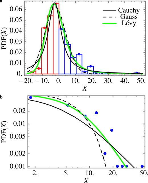
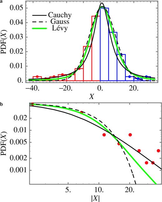
(a) The (discrete) probability density function (PDF; red and blue dots and bars) for the filtered strike slip X of the Hyogo-ken Nanbu (Kobe) earthquake is compared to curves of the three probability laws that best fit the PDF: the Cauchy law (black curve), the Gaussian law (dashed curve) and the Lévy law (green curve). The left side of the PDF (X < 0) is coloured in red while the right (X > 0) side is in blue. The magnitude of the random variables (filtered slip) is given by X. The width of the bar, corresponding to the increment used to estimate the PDF, is 4. For this case, the shape of the PDF illustrated in (a) is asymmetric with respect to its maximum and best fit by an asymmetric Lévy law with parameter β≠ 0 (see also the Appendix). The PDFs associated with Cauchy and Gauss laws are both characterized by curves symmetric with respect to its maximum. For this reason, the curves of the Cauchy and Gauss laws ‘overshoot’ the extreme events in the left tail of the computed PDF. (b) The right tails of the curves in (a) are illustrated on a log–log plot. Lévy and Cauchy PDFs are characterized by tails that decay according to a power law that is best illustrated on a log–log plot. The misfit of the Gaussian PDF is more obvious in this plot. In particular, note that according to the Gauss law, the large (filtered slip) values—last points on the right hand side of the graphics—have almost a zero probability of being observed. The parameters of the Gauss, Cauchy and Lévy laws are given in Table 2.
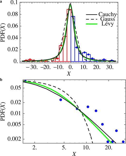
Same as Fig. 6, but for the random variables associated with the filtered strike slip of the Imperial Valley earthquake. The width of the bar, corresponding to the increment used to estimate the PDF, is 3. The remarks discussed in the caption of Fig. 6 (b) also apply for this case (see also Lavallée & Archuleta 2003). The parameters of the Gauss, Cauchy and Lévy laws are given in Table 2.
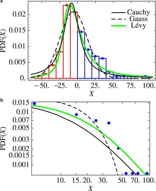
Same as Fig. 6, but for the random variables associated with the filtered strike slip of the Loma Prieta earthquake. The width of the bar, corresponding to the increment used to estimate the PDF, is 10. The remarks discussed in the caption of Fig. 9 for an asymmetric PDF also apply here. The parameters of the Gauss, Cauchy and Lévy laws are given in Table 2.
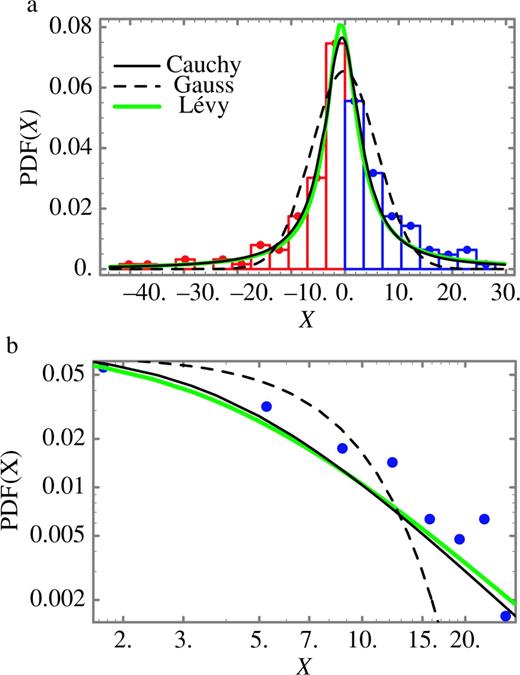
Same as Fig. 6, but for the random variables associated with the filtered strike slip of the Northridge earthquake. The width of the bar, corresponding to the increment used to estimate the PDF, is 4. The remarks in caption of Fig. 6(b) also apply for this case. The curve corresponding to the Lévy law underestimates the maximum of the PDF but provides a better fit to the other PDF values. The parameters of the Gauss, Cauchy and Lévy laws are given in Table 2.
The final step consists in determining the probability law that will provide the best fit to the PDFs illustrated in Figs 6–9. Three candidates are considered: the Gauss law, the Cauchy law and the more general Lévy law. The method to compute the parameters is discussed in the Appendix. For each earthquake, the parameters of the best fitting Gaussian, Cauchy and Lévy laws are listed in Tables 1 and 2. The curves of the Gaussian, Cauchy and Lévy laws that best fit the PDF are shown in Figs 6–9. For each slip distribution in this study, the Lévy law provided the best fit to the PDF. For almost all of the available slip distributions, the Cauchy law provides a better fit than the Gauss law except for the dip and strike slip of the Hyogo-ken Nanbu (Kobe) earthquake. In Figs 6–9, the tails of the PDF are compared to the tail of the best fitting Cauchy, Gaussian and Lévy curves, confirming that the Lévy law provides a better fit.
In computing the PDF associated with the Imperial Valley slip distribution (see Fig. 7), we purposely chose to compute the PDF for an increment in the random variable magnitude ΔX (corresponding to the width of the columns in Fig. 7) that differs from the one used in Lavallée & Archuleta (2003). The motivation for this choice is to get a rough estimate of the variation in the PDF parameters due to a change in the computed PDF. In Lavallée & Archuleta (2003), ΔX was set to 2.5 but is equal to 3.0 here. In this paper, we assume that the PDF is symmetric (β= 0); so only three parameters were determined. Comparing the values of the four Lévy parameters for width increments 2.5 and 3.0, we obtain, respectively, values of 0.92 and 1.14 for α, 0.0 and 0.04 for β, 3.75 and 2.75 for γ, and values of −1.0 and −0.42 for μ. The order of magnitude of each parameter is similar for both computations. These numerical computations give an indication of the accuracy of the parameters values estimated (see also the Appendix for questions related to the accuracy of the estimated parameters).
For the seven cases studied here, we find that the power spectrum behaviour can be approximated by a power-law behaviour, although the accuracy of this approximation varies from one case to another (see the discussion in the caption of Fig. 5). The 1-D power spectrum scaling exponent ν takes values between 0.78 and 1.71. For the three earthquakes for which analysis of slip in both the dip and strike directions are performed separately, we find that the scaling exponent values for the strike slip is systematically larger (see Tables 1 and 2); Mai & Beroza (2002) reached a similar conclusion. However, only the Northridge earthquake has a scaling exponent that varies significantly for the two directions (see Tables 1 and 2). This suggests a higher correlation in the strike direction with the implications that the scaling properties of the Northridge spectrum are anisotropic.
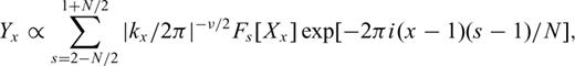
There are variations in the values of the Lévy parameters (Tables 1 and 2) computed for the seven cases we have examined. When comparing the values of the parameters α for the dip and the strike directions of these three earthquakes, we find no significant difference. The parameter α takes values close to 1, except for Hyogo-ken Nanbu earthquake, where the values are around 1.5. This suggests that the number of large slip events—asperities or large stress drops—is less frequent for this earthquake when compared to the other three earthquakes. The values taken by the parameter β indicate a significant departure from a symmetric PDF for both slip distributions (along dip and along strike) of the Loma Prieta earthquake and the strike slip of the Hyogo-ken Nanbu earthquake. For the Loma Prieta, Hyogo-ken Nanbu and the Northridge earthquakes, the values of the γ parameters associated with the dip slip are systematically larger that those computed for the strike slip. For both the dip slip and the strike slip, the values of γ decay from a maximum for the Loma Prieta earthquake, followed by the Hyogo-ken Nanbu and the Northridge earthquake. There is no simple interpretation of the variation in the values of γ when going from one earthquake to another, since one or several parameters of the stochastic model, such as α, β and ν, are also varying significantly from one model to another. (It should be noted that the values estimated for the parameter γ will depend on the definition adopted for the inverse Fourier transform used in eq. (4), but α is not affected by this definition.) Finally, note that when s= 1, the wavenumber k= 0 in the convolution given by eq. (4). This implies that the average value of the random variables estimated with eq. (4) will be zero. This will affect the values computed for the location parameter μ and suggests that not much importance should be assigned to the particular values of μ.
Variations in the stochastic model parameters from one earthquake to another may imply a dependence between the random properties of the earthquake and the physical properties of the fault. It may also point to some important difference in the process governing rupture propagation for each of the earthquakes. However, these variations may also reflect, at least partially, the presence of additional noisy effects and other uncertainties in the data. The slip models used in this study were determined using different algorithms. The algorithms themselves may be a cause for variations in the stochastic model parameters—for instance due to the inclusion of interpolation techniques (Liu & Archuleta 2004) or directivity effects (Sekiguchi 2002) in the inversion. Further investigations into the inversion methods would be needed to reach a definitive conclusion. Nevertheless, these results show that the stochastic model described at the beginning of this section, can be used to compute the one-point and two-point statistics of several earthquakes.
4 2-D Stochastic Model
4.1 Formulation of the stochastic model
In the previous section, we presented the results of our analysis of the statistical properties of the earthquake source models in terms of a 1-D stochastic model. The stochastic model is based on the assumption that the horizontal layers are statistically independent one from the other. This assumption is not completely accurate. For instance, a computation of the 2-D Fourier amplitude of the dip and strike slips of the Northridge earthquake suggests that the 2-D Fourier amplitude is a function of the wavenumber amplitude  , with k the 2-D wavenumber vector; kx and ky are horizontal and vertical wavenumbers, respectively (see Fig. 10). To investigate the dependence on the wavenumber amplitude, we can make the assumption that the slip distribution is isotropic and that the spectrum is only a function of k (see also Mai & Beroza, 2002 for a discussion on this issue). Consequently, this will imply that the correlation function—that is, two-point statistics—is only a function of the distance between the two points and not of the direction. This assumption, as the one discussed in the previous section, can be understood as a first order approximation. Both assumptions are probably too simple to fully account for all the complex features included in the slip model (see Fig. 10). As far as we know, there is no theoretical formulation available for the correlation function of the spatial slip distribution that goes beyond the model discussed in this section (see also Herrero & Bernard 1994; Mai & Beroza 2002). Furthermore, empirical derivation of a more sophisticated functional behaviour for the correlation function—or spectrum—is hardly possible due to the low number of subfaults computed in slip models. The only available alternative to the assumption that the horizontal layers are statistically independent is the assumption that the slip distribution is isotropic. In this section, we derive a stochastic model for the Northridge slip distribution based on the assumption that the correlation is isotropic. The goal of this exercise is to be able to appreciate the correctness of the description of the slip magnitude—that is, one-point statistic—in terms of a Lévy distribution under these two assumptions. We are also interested in comparing how the parameter values change as a function of the 1-D or 2-D description.
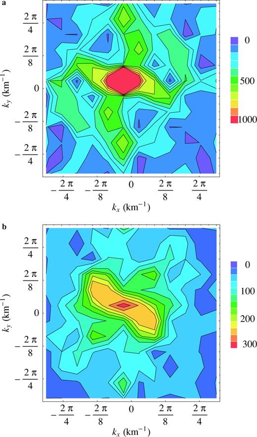
Contour plot of the complex behaviour of the Fourier amplitude of the dip (a) and strike (b) slip in the wavenumber space. The Fourier amplitude is function of the horizontal and vertical wavenumbers, respectively, kx and ky. The large and low values of the Fourier amplitude are in red and blue, respectively. However, in (b), contour lines are distributed almost horizontally in a region close to ky= 0, indicating higher correlation along this direction. This suggests that the approximation of the strike slip in terms of a 1-D stochastic model is more appropriate in this case (see Section 3).
 . Both sums in eq. (5) go from 1 to N; the discrete variables s and t are related to k by
  is the 2-D discrete Fourier transform of the random variables (for s≤ 0, the index s=N+s and for t≤ 0, the index t=N+t in Fs,t[Xx,y]). According to this formulation, the 2-D power spectrum density PD(k) for Yx,y will be given by the following relation (see Peitgen & Saupe 1988):
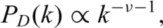
 (Parseval's theorem). (Note that integration over the azimuthal angle in the Fourier domain is included in PD(k)—see Turcotte 1997.) As for the 1-D stochastic model, after computing the scaling exponent ν for a stochastic model Yx,y, the random variables Xx,y can be computed by using the relationship:
4.2 Stochastic modelling of the 1995 Northridge slip distribution
Assuming an isotropic distribution of heterogeneities, we compute the 2-D power spectrum density, for the dip- and strike-slip distributions of the Northridge earthquake (Fig. 11). The values of the scaling exponents are close to 2 (Table 3). These values are in good agreement with the model of slip heterogeneity discussed by Lomnitz-Adler & Lemus-Diaz (1989). Based on a dimensional analysis of the slip property at different scales for such models, Herrero & Bernard (1994), inferred that the slip Fourier amplitude should decay with a power law given by k−1 and, thus, the power spectrum density will decay according to a k−2 power law. Herrero & Bernard (1994), discarded the Lomnitz-Adler and Lemus-Diaz's model on the basis that the stress drop values are not ‘physically suitable’ for the limiting cases of very large or very small values of k. This assertion need to be reexamined in view of the hypothesis that the power-law behaviour of the power spectrum density is limited to a finite range of k values (see Section 2).
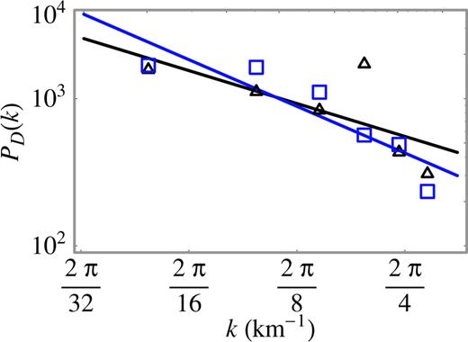
The 2-D power-spectrum density PD(k) is computed assuming that the dip and strike slip spatial distributions are isotropic. The square of the Fourier amplitude is estimated. The results are integrated over a (approximated) circle of radius k with 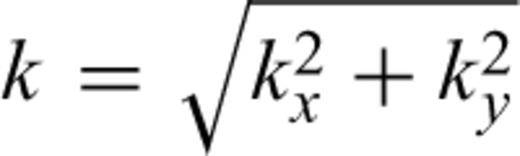 and then divided by k. The 2-D power-spectrum density PD(k) and the straight line that best fits the log–log curve are shown for the dip slip distribution (black triangle ▵), and the strike slip distribution (blue square
  ). These results suggest that the scaling behaviour is observed for a scale length ranging from 4 to 20 km. The values of the scaling exponent are given in Table 3. The linear correlation coefficient (in absolute values) takes a value of 0.91 for the dip slip and 0.96 for the strike slip.
Parameters of the 2-D stochastic model for the dip and strike slip of the Northridge earthquake. The parameter (ν+ 1) is the scaling exponent of the 2-D power-spectrum density (Fig. 14). The parameters of the Gauss, Cauchy and Lévy laws that best fit the PDF(X) in Figs 15 and 16 are given.
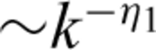 with the scaling behaviour generated by interpolation of the data ∼k
 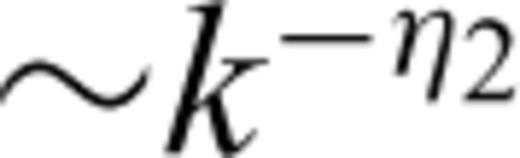 : that is the power spectrum would have the following relationship:
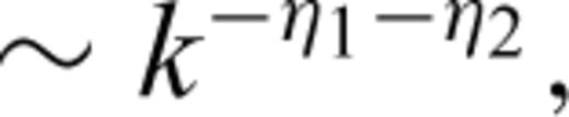
The spatial distribution of the random variable Xx,y is obtained by filtering in 2-D (see eq. 7) the slip distribution. The random variable is a slip that has a flat power spectrum. The (discrete) PDFs are computed for the filtered strike slip (Fig. 12). Finally, the parameters of the Gaussian, Cauchy and Lévy laws that best fit the PDF (Table 3) are computed following the procedure described in the Appendix. The discrete PDF as well as the curves of the Gaussian, Cauchy and Lévy laws that best fit the PDF are shown in Fig. 12.
Same as Fig. 6, but for the random variables correspond to the 2-D filtered strike slip of the Northridge earthquake. The width of the bar, corresponding to the increment used to estimate the PDF, is 8. The remarks given in the caption of Fig. 6(b) apply here. The parameters of the Gauss, Cauchy and Lévy laws are given in Table 3.
As was true for the 1-D modelling of the Northridge earthquake, the Lévy law again provides the best fit to the computed PDF. In 1-D and 2-D, the distribution of the random variables (the filtered slip) is almost symmetric (β close to 0). However, the parameter α takes larger values when compared to the values obtained for the 1-D modelling of the Northridge earthquake. Nevertheless, these values are within the range of values reported for all the earthquakes discussed in the previous section. This implies that the 1-D model predicts extreme large events—such as asperities—with a higher frequency than the 2-D model. It is difficult to assess the reason why we observe such a difference. This may reflect uncertainty in the estimate of the parameter α for this data set (see also the Appendix on this question). To get a better estimate of this parameter, and also to assess the correction of a 1-D or 2-D stochastic modelling, additional investigations are needed. For instance, one could analyse in parallel the statistical properties of the source model and the ground motion (see Lavallée & Archuleta 2005).
Comparison of the values of the parameters γ and μ obtained from a 1-D and 2-D modelling is not relevant (as described in the previous section). The value taken by the parameter γ depends on the constants used in the definition of eqs (2) and (5). These constants are not identical and have a different effect on the estimated γ.
The basic idea behind the wavenumber filtering is to obtain (iid) random variables (white noise) for which we can compute the probability law associated with them (see also the discussion in Section A2 of the Appendix). The random variables, computed through the 1-D and 2-D filtering processes described above, are only approximately independent and identically distributed. Nevertheless, the values of the parameters for the Cauchy, the Gauss and Lévy laws following the 1-D and 2-D filtering suggests the range of values that parameters of the Lévy law can take.
5 Discussion: Consequences of the Lévy Law
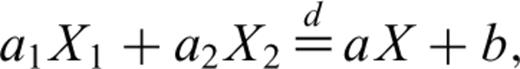
 stands for equal in probability distribution—that is, the random variables a1X1+a2X2 and aX+b have the same probability distribution or PDF. This implies that the PDF for X will differ from the PDF for X1 or X2 by a translation along the horizontal axis and a multiplicative constant (Uchaikin & Zolotarev 1999). This property was called ‘self-replication’ in Kagan (1994) since ‘the sum of random stable [Lévy] variables is itself a stable [Lévy] variable’.
For any (discrete) location on the grid, eqs (4) and (7) can be reduced to a sum of N (iid) Lévy random variables (weighted by constant). According to the Central Limit Theorem, the stochastic model Yx(1-D) or Yx,y(2-D) will have its amplitude distributed according to a Lévy law. Consequently, the slip or pre-stress spatial distribution is also distributed according to a Lévy law, although the parameters of the Lévy law—γ and μ—will be functions of the spatial position on the fault surface.
Consider now the operation of local averaging (also known as coarse graining)—that consists in computing an average over a space interval smaller than the total length of the grid but larger than the grid resolution. This operation applied to a stochastic model Yx corresponds to a sum of Lévy random variables (weighted by different constants). According to the Central Limit Theorem, the amplitude of the resulting field, at a lower resolution, will be also distributed according to a Lévy law, although again the parameters of the Lévy law—γ and μ—will be functions of the resolution. Slip models for different earthquakes are often computed at different resolutions. To get all the slip models at the same resolution, one can compute local averages over those models with a higher resolution. The statistical properties of the slip transformed under such an operation will not be affected. In other words, a description of the slip statistical properties in terms of the stochastic model discussed above guaranties that such properties are similar within the scales for which the spectrum power-law behaviour remains valid. Computation of the statistical properties of the slip distribution at different resolutions will become almost intractable if the statistical properties of the slip cannot be approximated by a Lévy law. The statistical properties, and in particular the probability law, will depend on the resolution of the slip inversion.
The dependence of the statistical properties of the slip distribution on the resolution of the slip model has been ignored most of the time. Neglecting this question has consequences that need discussion. Consider the converse by supposing that the slip or pre-stress spatial variability is distributed according to a non-Lévy law. For instance, let us assume that it is a uniform law. This is the hypothesis adopted by several authors to generate the slip heterogeneity (Boore & Joyner 1978) or the pre-stress heterogeneity (Oglesby & Day 2002). Under the Central Limit Theorem, a sum of (iid) random variables distributed according to a uniform law converges to a Gauss law. This implies that any transformation of slip—spatially distributed according to a uniform law—that involves a sum will lead to a slip that differs significantly, in terms of its probability law, from the original slip distribution. Examples of such transformations found in the literature include smoothing the slip (Oglesby & Day 2002) and using interpolations to get the field at higher resolution (Somerville 1999; Mai & Beroza 2002). Such transformations introduce an artificial dependency between the slip resolution and the probability law. A subsidiary question arises. Assuming that by inversion of ground motions one finds slip variability that is distributed according to a uniform law at a certain resolution, what kind of probability law will be found at a higher resolution? What kind of transformation is required to relate the probability laws computed at different resolutions?
In seismology, as in geophysics in general, data are collected or inferred at various resolutions either in time or space. To get a statistical description of the observation where the description is independent of the resolution imposes constraints on the choice of probability laws that can be used for such a purpose. If we do not want to specify different probability laws at different resolutions, the properties of the random variables should remain invariant under mathematical transformations that mimic transformations of data from one resolution to an other. Because of the Central Limit Theorem, the Lévy random variables have these properties.
The stochastic model discussed in this paper can also be used to generate synthetic slip spatial distributions. Several algorithms have been developed to generate Lévy random variables (Chambers 1976; Grigoriu 1995; Nikias & Shao 1995). Examples of synthetic fields generated by the stochastic model discussed above and comparisons to real data are discussed in Lavallée & Archuleta (2003). Detailed discussions of the procedure to generate fBm are available in the literature (see among others, Peitgen & Saupe 1988; Crilly 1991; Turcotte 1997). Substituting Lévy random variables for the Gauss random variables in these procedures will generate stochastic models equivalent to those given by eq. (2) or (5). Note, that because an interpolation in the physical space corresponds to extrapolation in the Fourier space, the stochastic model can be used to simulate spatial distributions of slip at a subresolution not currently available through kinematic inversions.
Accordingly, the stochastic model will allow one to generate many samples of slip spatial distributions. Although the samples are characterized by the same model parameters, every sample will be visually different from the others. This is a consequence of the random nature of the model. We also think that it is due to the intrinsic random nature of the earthquake process that source models computed for the same earthquake can be so different from one another. (Examples of different source models for the same earthquake can be found at the following address: ; Mai 2005.) For instance, consider the following experience where several dice are thrown but only the sum is recorded. Let us assume that, in addition to the number of dice, this is the only information made available to the modellers. Based on mechanical laws of motions, one can generate simulations of the rolling dice. For instance if for a pair of dice the observation is seven, then scenarios of rolling dice that provide final combinations, such as one and six, two and five or three and four, are all legitimate although quite different solutions. A similar interpretation may hold for the radiation field generated by the earthquake ruptures. Namely, several combinations of asperities distributed over the fault, statistically equivalent but physically located at different positions, can generate a seismic wave radiation pattern that is similar in terms of observations.
This section would not be complete without discussing the caveats and limitations underlying the results discussed in this paper. Ground motion is usually understood has a convolution of source, path and site effects. The inversion for the source model depends on the wave propagation through an uncertain crustal structure. The effect of this uncertainty is a fundamental but difficult question. In principle, uncertainties in the slip distribution can be partially quantified by comparing the slip distribution computed in different inversions. However, only a few papers have inverted real data using the same method applied to different velocity models (Ji 2002; Liu & Archuleta 2004). One can also argue that the quality of the available data is not sufficient, or that the number of subfaults is not large enough to achieve a significant description of the statistical properties of the source model. In the Appendix, we discuss the issues related to the computation of the statistical properties when there are a limited number of subfaults that describe the slip.
There is no doubt that the slip models are not perfect or that there are parts of the fault that are not well resolved. It should be noted that ‘lack’ of quality or resolution has not prevented using these slip models as a basis for numerical simulations of rupture propagation under heterogeneous conditions by which properties of the source have been inferred (e.g. Beroza & Mikumo 1996; Ide & Takeo 1997; Olsen 1997; Nielsen & Olsen 1999; Peyrat 2001; Ide 2002; Favreau & Archuleta 2003). The slip models remain a primary description of faulting that is derived from data. Our emphasis has been to find statistical parameters of the faulting that are consistent with the data.
The results, reported in Sections 3 and 4, are in good agreement with other results reported in the literature. For instance, in studies of the distribution of asperities over a fault, Fakao & Furumoto (1985) found that the probability (or complementary cumulative distribution function: equal to one minus the cumulative distribution function) for the size of the asperities is best described by a power-law behaviour with an exponent of 1; Gusev (1989), concluded that the exponent should be 2. Except for α= 2, that is, Gauss law, the Lévy complementary cumulative distribution function is characterized by a ‘heavy tail’ that follows a power-law behaviour with exponent α (see Uchaikin & Zolotarev 1999, among other). The values of α, given in Tables 1–3, are within the previously reported values of 1 and 2. In a subsequent paper, Gusev (1992) speculates on the Lévy law as a potential candidate to describe the asperity distribution. Furthermore, Kagan (1994) has suggested that in earthquake focal zones the stress increments due to past earthquakes are also distributed according to a Lévy law with α close to or less than 1 (on this question see also Marsan 2005). Ouillon & Sornette (2005) have used stress sources distributed according to a Cauchy law—as suggested by Kagan (1994)—to derive a new formulation of the Omori law. Finally, the computed parameters of the stochastic model for a source model of the 1999 Chi Chi earthquake are in good agreement with values reported in Section 3 (Lavallée & Archuleta 2005).
We have not included the spatial variation in other source parameters such as rise time and rupture velocity. Nor have we considered the effect of the time evolution of heterogeneity, for example, that may arise due to healing of the fault. The study of complexity in geophysics is a very difficult task. As far as we know, there are no guidelines or recipes that will guarantee success in deciphering complexity. In devising our strategy to investigate earthquake complexity, we first decided to try to isolate the effect of slip and pre-stress spatial heterogeneity. Spatial and time variability in other parameters as well as potential coupling effects between the parameters can be added in future research.
6 Conclusion
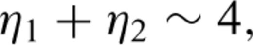
In this study, we have investigated the variability of slips models computed for four earthquakes: the 1979 Imperial Valley, the 1989 Loma Prieta, the 1994 Northridge and 1995 Hyogo-ken Nanbu (Kobe). For the four earthquakes, we show that the average 1-D power spectrum—and the 2-D power-spectrum density—of the raw, that is, non-interpolated, data follow a power-law behaviour where the scaling exponents have values less than −4 (see Tables 1, 2 and 3). These results suggest that the origin of correlations in computed slips models are not clearly understood and request additional investigations. In particular, going beyond the specificity of each algorithm used to compute source inversion, we should try to understand how the number, the location and configuration of stations used in the inversion (Custódio 2005) affect the random properties of the slip spatial variability in general, and the computed behaviour of the spectrum in particular.
Equally important to the wavenumber spectrum is the PDF for the filtered slip amplitudes. We find that the filtered slips are non-Gaussian; a Lévy law provides the best fit. Lévy laws are characterized by long probability tails that allow the presence of ‘extremes’, that is, large values of slip—corresponding to asperities—with a higher frequency of occurrence than with a Gaussian law. Our analysis implies that there is a higher probability of having large slip amplitudes distributed over the fault surface, for example, see Fig. 4 in Lavallée & Archuleta (2003) for a comparison between synthetic earthquake slip distributions based on random variables distributed according to a Cauchy law and a Gauss law. The effects of different distributions on rupture propagation are noticeable in movies of dynamic rupture (.) These results suggest that some features of the slip heterogeneity are quite general, perhaps ‘universal,’ and thus can be formulated in term of the stochastic model discussed in this paper.
For the Northridge earthquake, we considered two different assumptions regarding the properties of the spectrum or correlation function. Although in both cases we observe that the slip spatial variability can be approximated by Lévy random variables, the parameters of the Lévy law depend on the filtering necessary to obtain the white noise. It should be noted, however, that the variation in values derived from the data for the Lévy index parameter α—the parameter characterizing the fall off of the PDF for large event—is of the same order of magnitude as the variation observed in this parameter from computer generated Lévy random variables (see the Appendix).
The randomness of the source has been postulated in several papers, and in a fewer number of papers, stochastic models have been inferred and parametrized through comparison with data. There is a consensus that, as far as earthquakes are concerned, nature is indeed rolling dice. The results presented in the present paper confirm that it is the case but with one important qualification: the probability law that governs the statistics of the dice is a Lévy law.
Acknowledgments
We appreciate the valuable comments and constructive criticism of the reviewer P. M. Mai and an anonymous reviewer. We would like to thank H. Sekiguchi for kindly providing the source model for the 1995 Hyogo-ken Nanbu (Kobe) earthquake, and J. Steidl for the source model for the 1989 Loma Prieta earthquake. We also thank J. C. Nave for helpful discussions. This research has been supported by SCEC grant No. 572726 as well as UCSB matching funds for SCEC, KECK grant No. 19990997, and LANL/IGPP grant No. 04-08-16L-1532. SCEC is funded by NSF Cooperative Agreement EAR-0106924 and USGS Cooperative Agreement 02HQAG0008. This is SCEC Contribution No. 871. This is ICS contribution No. 0688.
References
Appendix
Appendix A: On the Estimate (Determination) of the Parameters of the LÉvy Law
A1 White noise
In this appendix, we discuss the procedure used to estimate the Lévy parameters corresponding to a set of random variables. We also present the results obtained when using this procedure on Lévy random variables generated with the proper algorithms. However, first, we have to introduce the mathematical formulation of the PDF and characteristic function for the Lévy law (detailed discussions can be found in the literature: Feller 1971; Grigoriu 1995; Nikias & Shao 1995; Uchaikin & Zolotarev 1999; Sornette 2004).


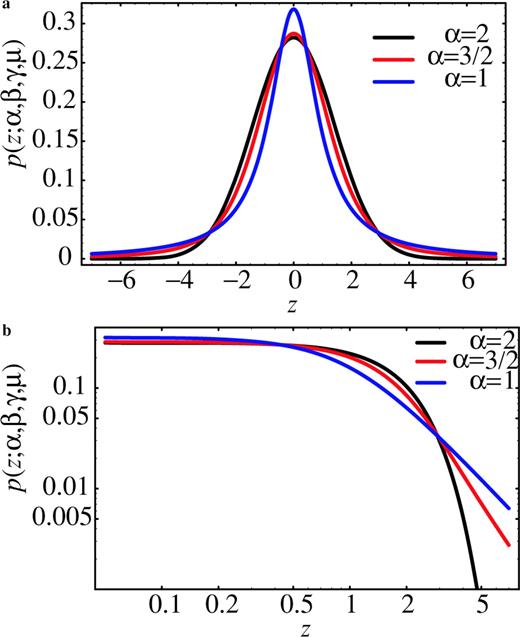
Curves of the Lévy PDF p(z; α, β, γ, μ) for several values of the parameter α: (a) the overall PDF and (b) the tails of the PDF. The parameter α is known as the Lévy exponent, the characteristic or stable exponent. It controls the rate of fall off of the PDF as illustrated in (b) on a log–log plot. Note that by keeping the values of other parameters fixed, the probability of observing random variables with large values increases as α decreases.

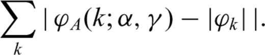
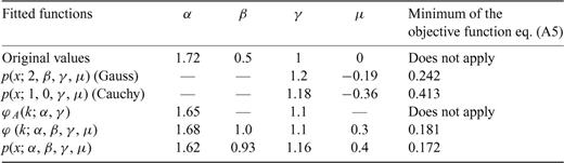
Compute the parameters γ and μ that optimize expression (A5) for a Gauss and a Cauchy law. In this computation, we use the well-known analytical expressions for the Gauss p(z; 2, 0, γ, μ) and Cauchy p(z; 1, 0, γ, μ) PDFs.
Compute the parameters α and γ that optimize expression (A9). For this purpose, we use as initial values for α and γ the values obtained in the first step, either the Gauss or Cauchy parameters depending on which one provides the lowest value for the objective function in expression (A5).
Compute the parameters α, β, γ and μ that optimize expression (A6). For initial values of α, β, γ and μ we use the values computed in the second step and the first step.
Compute the parameters α, β, γ and μ that optimize expression (A5). For initial values of the parameters to be determined we use those obtained in the third step.
Note that intermediary steps can be added to this procedure. For instance, in steps 3 or 4, one can use the value of α and γfound in the second step and optimize expressions (A5) or/and (A6) to fit only the parameters β and μ. If the computer is too slow, one can consider replacing step 4 by this variation. (For instance, computing the step 3 with a 360 MHz Sun Ultrasparc station takes 18768 seconds of CPU time, while it takes 2531 s with a 1 GHz G4 Titanium Apple Powerbook and 855 seconds with a 2Ghz Dual G5 Apple Desktop. Computing the step 4 (for the same data) takes 10 005 ss of CPU time with a 2Ghz Dual G5 Apple Desktop.) To provide robust results, it is better to perform the computation for different sets of initial values of the parameters. This will also ensure (as much as possible) that the optimization compilation is not trapped in a local minimum. For the three last steps, we use the Mathematica algorithm NMinimize for all the results presented in this paper, with the three methods for global optimization: genetic programming, non-linear simplex algorithm and simulated annealing. For the first step, we either use NMinimize or NonlinearRegress.
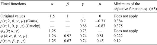
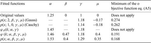
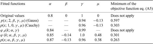
To assert its soundness, the procedure to compute the Lévy parameters has to be tested. Furthermore, the procedure has to be tested under conditions that are as close as possible to the conditions used to compute the Lévy parameters corresponding to the slip distribution. For this purpose, we have generated 200 Lévy random variables (white noise) using the algorithms discussed in Chambers (1976) and Grigoriu (1995) with different values for the parameters α, β, γ and μ. (These algorithms should be used carefully, because depending on the seed and the number of random variables generated, convergence toward the theoretical distribution is not automatic.) The number of random variables is chosen to match roughly the number of events (subfaults) used in the analysis of the slip spatial distributions: 144 (Loma Prieta), 180 (Northridge), 196 (Imperial Valley) and 280 (Hyogo ken Nanbu -Kobe). The PDF and the characteristic function—see eq. (A7)—corresponding to these random variables are computed. (When fitting the PDF and the characteristic function of the white noise or filtered slip, we neglect that the computed PDFs for the white noise or filtered slip are truncated.) Then, the procedure discussed above is used to compute the best-fitting values for the parameters α, β, γ and μ. Comparisons between the best-fitting values computed at each iteration and the original values used to generate the random variables are presented in Tables A1 to A7—see also Fig. A2. In Tables A3 and A4, the values of the parameters are identical even though the algorithm used to generate the Lévy random variables is different: the algorithm of Chambers (1976) for Table A3 and the algorithm given in Grigoriu (1995) for Tables A4 to A7. These results indicate the order of accuracy that can be expected for the parameters when considering two different samples of two hundred (iid) Lévy random variables.
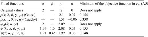
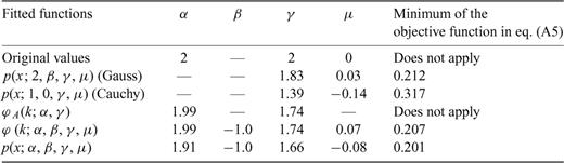
Summary of the values obtained for the parameters of the Cauchy, Gauss and Lévy law. The last column reports the values computed for the objective functions given in eq. (A5). Note that, although we report the values for eq. (A5) in the sixth line, the parameters reported in these lines were computed by optimizing eq. (A6). The second line includes the values of the Gauss parameters used to generate the random variables with an algorithm provided with Mathematica.
Same as Table A1. The second line includes the values of the Cauchy parameters used to generate the random variables with an algorithm provided with Mathematica.
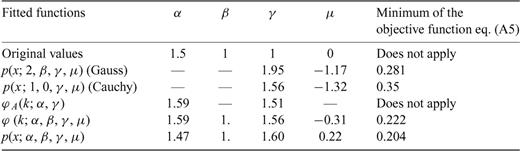
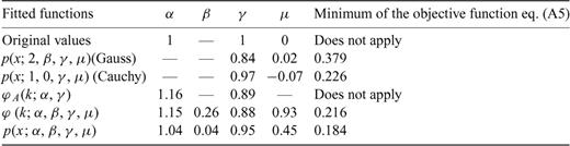
Same as Table A1. The second line includes the values of the Lévy parameters used to generate the random variables with an algorithm discussed in Chambers (1976).
Same as Table A1. The second line includes the values of the Lévy parameters used to generate the random variables with an algorithm discussed in Grigoriu (1995).
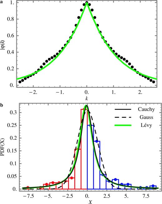
(a) Using eq. (A7), the absolute value of the characteristic function |ϕk| is computed for random variables distributed according to a Cauchy law (see Table A2, second row). The continuous (green) curve corresponds to the Lévy law that best fits |ϕk| in eq. (A9). The parameters of the Lévy laws are given in Table A2 (fifth row) (b) The (discrete) probability density function (PDF; red and blue dots and bars) corresponding to the random variables X discussed in (a). The curves of the three probability laws that best fit the PDF: the Cauchy law (black curve), the Gaussian law (dashed curve) and the Lévy law (green curve) are also shown here. The parameters of the Gauss, Cauchy and Lévy laws are given in Table A2 (in the third, fourth and last rows, respectively).
Note that when comparing the minimum of the objective functions reported in Tables A1 to A7 for a Gauss or Cauchy law to the minimum computed for a Lévy law, these values should be understood as indicative of only the relative quality of the fit not a definitive measure. A more accurate measure will require taking into account that two parameters are needed to fit a Gauss or Cauchy law while four are needed to fit a Lévy law. However, when comparing the fit of the Gauss law to the fit of Lévy law, the misfits of the PDF values located in the curve tail should be given a proper weight, because it is for these values that the Gauss law differs significantly from the Lévy law. (The misfits for the values located in the curve tail have a smaller contribution to the objective functions than the misfit near the maximum of the PDF. This is due to the fact that the PDF values near the curve maximum are larger in magnitude than the PDF values located in the tail of the curve.) Thus, a better quantification of the quality of the fit of the PDF tail will also require weighting accordingly the values located in the PDF tail. Adding these refinements to the analysis performed in this paper will not modify the conclusions.
The tests done using the procedure outlined above allow us to draw some conclusions. In general, the values for the parameters γ and μ that, respectively, characterized the dispersion and location of the PDF, are well estimated in term of their order of magnitude. This conclusion holds independently of the law or method used to estimate the parameters. For most of the studies, the procedure provides accurate values of the parameter α as long as the values of α are not too low. (For a set of two hundred variables, it is more difficult to approximate the theoretical behaviour of the PDF when α≈ 0.7 or smaller.) Of all the four parameters, β is the parameter estimated with the least accuracy, although the parity is usually well resolved. Thus the asymmetry or symmetry of the PDF curves is not well resolved for the number of random variables used in these tests.
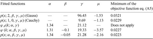
The question of how many random variables are needed to get an accurate estimate of the PDF and of the PDF parameters is beyond the scope of this paper. What we want to establish in this Appendix, is that given a number of random variables similar to those used in computing the stochastic model of the slip distributions and using a similar procedure, it is possible to discriminate between white noise distributed according to a Gaussian (α= 2), a Cauchy (α= 1, β= 0) and a Lévy (with a stable parameter value α not too close to 1 or 2) law. The study suggests that the parameter α can be estimated with an uncertainty of roughly ±0.3 (see Tables A4 and A5). This precision is for white noise, that is, generated (iid) random variables. For random noise obtained through the filtering of the slip distributions, the uncertainty is surely larger although not easily quantified (see the next section). These results suggest that the uncertainty of the values of α reported in Tables 1 to 3 is at least of the order of ±0.3. Within this margin of error, it is possible to distinguish between a Cauchy (α= 1) and a Gaussian (α= 2) random law. For the sake of comparison, with results presented in Tables A1 to A7, we present in Table A8 the results of the procedure outlined above for the dip slip of the Northridge earthquake.
Same as Table A1 but for the random variables corresponding to the dip slip of the Northridge earthquake.
Finally, the computed values for the parameters of the Cauchy, Gauss and Lévy laws depend to a certain extent on the size of the increment ΔX used to compute the PDF(X). However, numerical compilations of the parameters of the Cauchy, Gauss and Lévy laws for a reasonable choice of ΔX show that there is no significant change in the parameter values. For instance, the values presented in Table A8 are computed for ΔX= 7. Using a ΔX= 8 to compute the PDF(X), we obtain that the Gauss law is best fit for γ= 96.14 and μ=−1.55; the Cauchy law is best fit for γ= 10.35 and μ=−1.72; and the Lévy law is best fit for α= 1.28, β= 0.14, γ= 18.34 and μ= 0.76. These values are in good agreement with those reported in Table A8. That is, the results presented in Tables 1, 2 and 3, indicating that the Lévy law provides a better fit, are not an artefact that can be eliminated by choosing another reasonable value for ΔX. By reasonable value of ΔX we mean a value as small as possible—to get as many points as possible to fit the three probability laws—but large enough to reproduce the regular smooth shape associated to a PDF. There is no optimal way to make such a choice for ΔX, and it may be possible to get better results by using a variable ΔX. For N random variables Xi we perform the following comparison to insure a reasonable choice of ΔX. First we compute the mean directly from the data, using  , and compare to the mean computed with
  , using the computed PDF(X) at a given ΔX. Then, we compute the moment of second order directly from the data, using
  , and compare with the moment of second order computed with
  . The increment ΔX is chosen in such a way that both comparisons give similar values for the mean and the second order moment.
A2 Pseudo-white noise
In the previous section, we discussed the computation of the parameters of the Lévy law for a sequence of (iid) random numbers—white noise. For the slip distribution, we have to filter the data to approximate a white noise (see eq. 4 or 7). It should be noted here that in addition to having a flat spectrum (for instance ν= 0 for 1-D analysis), a second condition is necessary to insure that the filtered slip corresponds to a white noise: the parameter of the probability law should be invariant under translation across the filtered slip. Due to the number of subfaults found in a source inversion, it is hardly possible to verify—even as an approximation—the second condition. A related issue has to do with the accuracy of the scaling exponent computed for the slip distribution. In practice, to observe the theoretical scaling exponent corresponding to a random walk or fractional Brownian motion (with a Gauss or Lévy law), many samples of the stochastic model have to be generated. Spectrum analysis is performed on every sample, and computing the average power spectrum over all the samples usually allows recovery of the theoretical scaling exponent. To illustrate this issue, for each sequence of random variables already discussed in Tables 1–3 (corresponding to Gauss, Cauchy and Lévy with α= 1.5 random variables), we distribute the random variables on ten layers with twenty events (or subfaults). Each layer is then filtered using eq. (2) with ν= 1. We compute the scaling exponent to the average power spectrum as we did for the earthquakes source models discussed in Sections 3.2. We obtain the following values for ν: 1.09, 1.29 and 1.06 for Gauss, Cauchy and Lévy with α= 1.5 random variables.
For each case, using the estimated ν and eq. (4), we compute a pseudo-white noise. For each sequence of the pseudo-white noise, we compute the parameters of the Lévy law following the procedure outlined in the Section A1. The results are reported in Tables A9–A11. Comparing the results in Tables A9–A10 to those in Tables A1–A3, suggests that only the parameter γ is significantly different for the pseudo-white noise. (We already have noted in Section 3.2 that the value obtained for this parameter depends on the definition of the inverse Fourier transform used in eq. 4). Note also that the error in estimating the parameter α for the pseudo-white noise is within ± 0.3 of the input values. For most of the values reported in Tables A9 to A11, the values of the parameter α is in very good agreement with the corresponding estimates in Tables A1, A2 and A3. The good agreement obtained for α can be understood as a consequence as of the Central Limit Theorem (see Section 5 and Lavallée & Archuleta 2005).
Summary of the values obtained for the parameters of the Cauchy, Gauss and Lévy law for the pseudo-white noise. These results should be compared with the results obtained for the original white noise given in Table 1.

Summary of the values obtained for the parameters of the Cauchy, Gauss and Lévy law for the pseudo-white noise. These results should be compared with the results obtained for the original white noise given in Table 2.

Summary of the values obtained for the parameters of the Cauchy, Gauss and Lévy law for the pseudo-white noise. These results should be compared with the results obtained for the original white noise given in Table 3.
Based on these computations, it is possible to obtain reliable estimate of the parameters α, β and μ with a pseudo-white noise (that is, within the qualifications discussed elsewhere in this paper). However, it should be noted that this study is not exhaustive and should be considered as only indicative of the accuracy that can be achieved by analysing the pseudo-white noise in place of a real white noise.
