


Abstract
This paper presents a generalized wave equation which unifies viscoelastic and pure elastic cases into a single wave equation. In the generalized wave equation, the degree of viscoelasticity varies between zero and unity, and is defined by a controlling parameter. When this viscoelastic controlling parameter equals to 0, the viscous property vanishes and the generalized wave equation becomes a pure elastic wave equation. When this viscoelastic controlling parameter equals to 1, it is the Stokes equation made up of a stack of pure elastic and Newtonian viscous models. Given this generalized wave equation, an analytical solution is derived explicitly in terms of the attenuation and the velocity dispersion. It is proved that, for any given value of the viscoelastic controlling parameter, the attenuation component of this generalized wave equation perfectly satisfies the power laws of frequency. Since the power laws are the fundamental characteristics in physical observations, this generalized wave equation can well represent seismic wave propagation through subsurface media.
INTRODUCTION
For seismic wave simulation, there are two basic types of wave equations: pure elastic wave equation and viscoelastic wave equation. This paper proposes to unify these two types of wave equations into a single wave equation.
The mathematical-physics history of this empirical method, using a fractional derivative to represent the viscoelastic property, begins with Nutting (1921) who reported the observation that the stress relaxation could be modelled by fractional powers of time. Such a model is in sharp contrast to the traditional view that stress relaxation is best described by decaying exponentials. Gemant (1936) further observed that the stiffness and damping properties of viscoelastic materials appeared to be proportional to fractional powers of frequency. Scott-Blair (1947) pioneered a framework which used fractional order temporal derivatives to model simultaneously the observations of Nutting (1921) and Gemant (1936). Then, Caputo (1966, 1967) used the fractional order derivatives to model the viscoelastic behaviour of the earth's subsurface media.
Eq. (2) is identical to or almost identical to, respectively, all of the fractional calculus relationships reported in the literature (Caputo 1967; Caputo & Mainardi 1971; Bagley & Torvik 1983; Szabo 1994; Mainardi & Tomirotti 1997; Wismer 2006; Holm & Sinkus 2010; Jaishankar & McKinley 2013; Näsholm & Holm 2013). When the fraction β equals to 1, eq. (2) reduces to eq. (1), in which the viscoelastic model becomes Newtonian viscous model (Ricker 1943). However, when the fraction β equals to 0 and the viscosity is zero-valued, eq. (2) becomes σ(t) = (E0 + E1)ε(t), which is not the pure elastic model. Because eq. (2) cannot represent the pure elastic case, then the derived wave equation lacks generality for seismic waves.
This paper attempts to unify the viscoelastic and pure elastic cases into a single model. In this unified model, β still varies between 0 and 1. But, when the fraction β equals to 0, the model is able to represent any pure elastic media. The unified model leads to a generalized wave equation, for which an analytical solution is derived explicitly in terms of the attenuation and velocity dispersion. Moreover, this paper proves that the attenuation component of the unified wave equation follows power laws. The power-law attenuation is a fundamental characteristic, observed from many measurements and is reported in the vast body of the published literature. Therefore, this generalized wave equation can perfectly represent seismic wave propagation through subsurface media.
GENERALIZED WAVE EQUATION
This section unifies wave equations for the pure elastic and viscoelastic cases into a single wave equation.
Unified elastic-viscoelastic model
In this constitutive equation, for the unified elastic-viscoelastic model, the β factor pre-multiplied to the viscoelastic term is a combining factor in order to balance the elastic and the viscoelastic characteristics. We introduce the combining factor β here to ensure that eq. (6) is a pure elastic model when β = 0 and a linear viscoelastic model when β = 1.
The combining factor
Fig. 1 illustrates this f(β, q) coefficient in two cases: q = β (solid curves) and q = 1 (dotted curves). Each case displays two numerical examples with ω/ω0 = 0.5 and 2, respectively. In the case where q = β (the solid curves), eq. (6) approaches the pure elastic model, |σ(ω)| = |Eε(ω)|, when β → 0. However, for the case of q = 1 (the dotted curves), which is the commonly used case, eq. (7) approaches |σ(ω)| = 2|Eε(ω)| when β → 0. The latter is not the Hookean elastic model.

The square root coefficient f(β) in the viscoelastic model: comparison between the case with the combining factor q = β (solid curves) and the case q = 1 (dotted curves). Each case displays two numerical examples with ω/ω0 = 0.5 and 2, respectively.
For generality, the combining factor q can be set as a β-dependent function, such as q = βa, where a is a non-zero value. We have tested q = β1/2 and q = β2 (results not shown) and found that q = β is the best for balancing the elasticity and the viscosity in the model.
The wave equation
Although various constitutive viscoelastic equations may lead to different forms of wave equation (Holm & Näsholm 2014), the combination between the elastic model and the viscoelastic model should be the same as proposed in this paper.
THE ANALYTICAL SOLUTION
This section derives explicitly an analytical solution to the generalized wave equation.
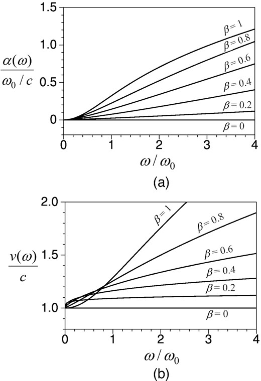
(a) The attenuation versus the β values. The horizontal axis (ω/ω0) is normalized frequency and the vertical axis is the attenuation α(ω) normalized by ω0/c, which has physical units of inverse distance. (b) Velocity dispersion versus the β values. The vertical axis is the phase velocity v(ω) normalized by the velocity c.
If β = 0, it is easy to verify that α(ω) = 0 and v(ω) = c. This is a pure elastic case. However, for the conventional equation in the previous body of literature, where the combining factor is q = 1, rather than q = β in eq. (11), eq. (22) will lead to v(ω) ≠ c when β = 0. This emphasizes the necessity of the combining factor β introduced in wave equation (11).
POWER LAWS FOR THE ATTENUATION
A fundamental characteristic of the viscoelastic media is that the attenuation satisfies power laws of frequency, for both compressional and shear waves (Collins & Lee 1956; White 1965; Kibblewhite 1989; Szabo & Wu 2000; Gómez Álvarez-Arenas et al.2002; Fabry et al.2003; Nicolle et al.2005; Kelly & McGough 2009; Treeby et al.2010). In this section, we will demonstrate that the generalized wave equation has a solution of attenuation that satisfies the power laws and is consistent with many laboratory measurements. We will also propose a general power-law form which is applicable to both low and high frequencies simultaneously, for any given β parameter.
One of the physical meanings of the power-law form in eq. (29) is that, for a weak viscoelastic case with a small β value, the attenuation is a linear scaling with frequency. Kibblewhite (1989) suggested that there are two mechanisms responsible for the attenuation. The primary mechanism is called ‘internal friction’ which somehow gives rise to a linear scaling with frequency, as in dry materials. The additional mechanism, due to the viscosity of the pore fluid, is responsible for any deviation from the linear power law in saturated materials.
As shown in Fig. 3(a), in the case where β ≥ 0.6, the attenuation for low frequencies approaches to the (1 + β)-, (1 + 2β)- and (1 + 3β)th powers of frequency, and eq. (28) is a modification of the second power of frequency. The latter is consistent with Biot's attenuation theory at low frequencies (Biot 1956a). Fig. 3(a) indicates that this frequency-square property is valid up to ω < 2ω0 for β = 0.6 and ω = ω0 for 0.8 ≤ β ≤ 1.0.
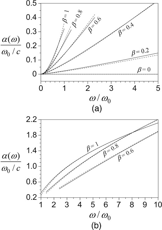
The attenuation follows the power law, whenever (a) |β(ω/ω0)β| ≤ 1 and (b) |β(ω/ω0)β| > 1. The solid curves are the exact solution and the dashed curves are the power-law approximation. The vertical axis is the attenuation normalized by ω0/c.
The series of coefficients λn in the power-law formula can be determined numerically, for any given β value (0 < β ≤ 1). Whenever sin (nβπ/2) = 0, for example, (β, n) = (4/5, −5/2), and (β, n) = (1, 2), we set λn = 0 and estimate the rest. Table 1 summarizes coefficients λn for the power-law form in eq. (32).
The coefficients in the general power-law form for the attenuation.
| λn (β = 0.1) | λn (β = 0.2) | λn (β = 0.3) | λn (β = 0.4) | λn (β = 0.5) | |
|---|---|---|---|---|---|
| n = −11/2 | 0 | 0 | −0.000042 | 0.000353 | 0.000508 |
| n = −9/2 | 0.000002 | 0.000021 | 0.000465 | 0.004995 | −0.019584 |
| n = −7/2 | −0.000013 | −0.000754 | −0.002632 | −0.007785 | −0.116293 |
| n = −5/2 | −0.000338 | 0.005661 | 0.007857 | −0.003614 | 0.131893 |
| n = −3/2 | 0.005620 | 0.000697 | −0.006141 | 0.110538 | −0.157434 |
| n = −1/2 | −0.010068 | −0.338306 | −0.075679 | −0.717437 | 0.066795 |
| n = 1 | 0.809407 | −0.136882 | 0.325118 | −0.258210 | 0.224411 |
| n = 2 | 0.086575 | −0.649135 | −0.169018 | 0.200912 | −0.056932 |
| n = 3 | −2.767400 | 1.170922 | 0.063227 | −0.070068 | 0.008822 |
| λn (β = 0.6) | λn (β = 0.7) | λn (β = 0.8) | λn (β = 0.9) | λn (β = 1.0) | |
| n = −11/2 | 0.000627 | −0.000585 | −0.001013 | 0.000335 | −0.000019 |
| n = −9/2 | −0.010728 | 0.003230 | −0.014219 | −0.095917 | −0.001965 |
| n = −7/2 | 0.393432 | −0.043753 | 0.034206 | −0.067135 | −0.042692 |
| n = −5/2 | 0.264238 | −0.338536 | 0 | 0.732270 | 0.293508 |
| n = −3/2 | −0.269011 | 0.318444 | 0.239684 | 0.740397 | 0.863421 |
| n = −1/2 | 0.273594 | −0.752771 | −0.706726 | −1.065600 | −1.071839 |
| n = 1 | 0.318932 | 0.0426558 | 0.043124 | −0.001986 | −0.001549 |
| n = 2 | −0.110450 | −0.013564 | −0.016306 | 0.000316 | 0 |
| n = 3 | 0.047285 | −0.006779 | −0.001231 | −0.000003 | −0.000006 |
Table 1 lists the nine coefficients for each case with a constant β value. Because those additive terms in eq. (32) are not orthogonal to each other, using more or less terms in curve fitting will alter the estimated coefficients listed in the table. The 9-term generalized power-law formula in eq. (32) can fit both low and high frequencies with sufficient accuracy. This is certainly an advantage over any conventional analysis conducted over separated regimes (Holm & Näsholm, 2011, 2014).
In Table 1, the coefficients are estimated from an individual attenuation curve of a single β constant. If different attenuation curves corresponding to different β values are combined into a single group for the coefficient evaluation, it will severely compromize the accuracy of curve fitting. Each group of coefficients is fitted to a wide range of frequency variation, up to 10 times the reference frequency ω0. In Fig. 4, power-law (black dotted) attenuation curves are overlaid with the (grey solid) curves of the analytical attenuation. The rms error for each case is <0.0015.
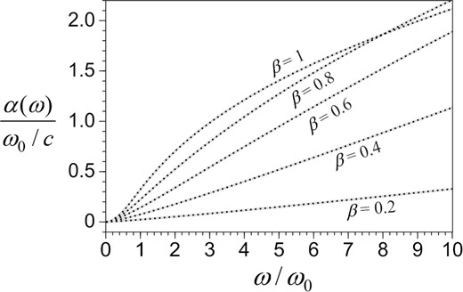
The analytical solutions of the attenuation are fitted by the power law. The grey solid curves are the analytical solutions and the black dotted curves are the power-law approximations. They match each other perfectly.
The wave dynamic properties (the attenuation and phase velocity) can be related to the mechanical properties (permeability, grain size, density and porosity) of a sediment (Hovem and Ingram 1979; Buckingham 1997). These power-law functions will be very useful for extrapolating laboratory measurements from an intermediate–high frequency range to a low-frequency range.
CONCLUSIONS
This paper has proposed a generalized wave equation which covers the viscoelastic case and the pure elastic case in a single equation. The parameter (β) controlling the degree of viscoelasticity also balances the characteristics between the elasticity and the viscoelasticity of the subsurface media. The analytical solution of the generalized wave equation is expressed explicitly in terms of the attenuation and the velocity dispersion.
This paper has also proved that the attenuation component of the generalized wave equation, defined by any constant β parameter, satisfies the power law of frequency. Since the power-law form is a general physical observation of the attenuation depending on the frequency, this generalized wave equation can well represent wave propagation in subsurface media. The theoretical solution might lead to a generalized definition of seismic wavelets (Wang 2015).
The author is grateful to the National Natural Science Foundation of China (Grant No. 41474111), and the sponsors of the Centre for Reservoir Geophysics, Imperial College London, for supporting this research.
REFERENCES
