


Summary
1-D reflectivity method in the frequency ray-parameter domain is the most popular method for computing synthetic seismograms. We explore an extension of this method to media consisting of homogeneous layers with curved interfaces. The 2-D extension of the method involves explicit evaluation of boundary conditions that results in a matrix formulation involving several matrix inversions in a coupled ray-parameter domain. First, we revisit this method by examining the intermediate results in the coupled shot-receiver ray-parameter domain for realistic models; numerous numerical artefacts are caused by matrix operations. Next we investigate an alternate asymptotic approach by examining a tangent plane or Kirchhoff formulation in the plane wave domain to replace the exact boundary condition evaluation. All other reflectivity operations such as the invariant imbedding or iterative computation of reflection, transmission, multiple and mode conversions can be readily applied even under this approximation. Our resulting algorithm computes noise free seismograms even with coarse sampling of the interfaces and ray parameters. Approximate calculation of reflection/transmission coefficients, however, does not include multiple interaction of a plane wave with an interface.
We show examples of synthetic seismograms for a suite of realistic models. Our computations are performed in the coupled slowness domain and thus, multiple shot-receiver data can be synthesized rapidly. Intermediate results in the coupled slowness space provide important insight into understanding wave propagation in heterogeneous media.
1 Introduction
Seismic modelling is essential for the interpretation and inversion of seismic data, and for generating synthetic data to test seismic processing algorithms. Several algorithms exist for forward modelling of seismic data depending on the accuracy of the solution and assumptions on the model. The ray-based methods generate asymptotic solutions at infinite frequency and can be applied to models of general complexity as long as rays can be traced through the medium (Cerveny 1985, 2001). Pure numerical methods based on finite difference (Virieux 1984, 1986) and finite element (Marfurt 1984) approaches generate complete solutions but these methods become prohibitively expensive at high frequencies. The reflectivity method that is valid for 1-D models and finite difference method valid for a general 3-D model, are the most popular methods for seismic modelling.
The reflectivity method (Fuchs & Mueller 1971; Kennett 1983) has been immensely successful in describing propagation of waves up or down a stack of elastic horizontally stratified (1-D) media. Extension of this approach to layered media in which velocities vary laterally (2-D, Koketsu 1987; Koketsu et al. 1991), however, is not used routinely in spite of the rigor and elegance of the method in the coupled slowness or wavenumber domain. The prime reason is that the 2 × 2 reflectivity matrices in 1-D case become 4N × 4N (P−SV) and 2N × 2N (SH), where N is the dimensionality of the discrete wavenumber space. The computation of reflection and transmission coefficients in laterally varying media requires at least one such matrix inversion at every interface (requires more number of matrix inversions for interbed multiples) and hence the complexity and errors grow with each recursion for propagation through a stack of layers. Most published examples include seismograms for a single incident plane wave from below a heterogeneous zone.
Ray methods are simple, intuitive and easy to implement. However, ray theory breaks down at caustics and other critical regions. Several methods have been proposed to modify the ray-based methods—they include extended WKBJ theory (Frazer & Phinney 1980; Chapman & Drummond 1982), Gaussian beams (Popov 2002) and Kirchhoff-Helmholtz methods (Frazer & Sinton 1984). Frazer and Sen, in a series of papers (Frazer & Sen 1985; Frazer 1987; Sen & Frazer 1991), formulated elastic Kirchhoff-Helmholtz (KH) integral approach in the frequency domain to calculate synthetic seismograms. In their formulation, the source and the receiver wavefields are expanded in a series of generalized rays through layers with irregular interfaces and then KH theory is applied to determine the coupling between each source ray and receiver ray at each interface. A tangent plane or Kirchhoff approximation is used to determine the coupling. The method essentially uses a combination of KH theory and geometrical optics between interfaces and plane wave reflection and transmission coefficients to propagate them across the interfaces. This method was extended to multilayered media into a multiple integral form called multifold path integral (MFPI). To improve on the Kirchhoff approximation further, the MFPI method was further extended to decompose the general source and receiver wavefields in a series of plane waves resulting in multifold ‘phase space path integral (PSPI)’ (Sen & Frazer 1991).
In a recent work, it has been shown (Sen & Pal 2007) that the 2-D reflectivity methodology can be effectively utilized to simultaneously obtain (1) plane wave seismograms τ-p-p′ in the coupled ray-parameter domain, (2) familiar τ-p seismograms at different locations along a profile and finally (3) the conventional ‘shot records’ in t-x-x′ domain where x and x′ denote the shot and receiver positions, respectively. This semi-analytic approach has the potential to be cost-effective in many applications. However, marching through successive layers involves multiplication and inversion of high-dimension matrices, which make the methodology unstable and error-prone after two or three general curved interfaces. Even for a single interface dipping uniformly in one direction—the simplest deviation from a flat interface—the theoretically elegant 2-D reflectivity method encounters problems because it turns out that the matrix required for inversion have non-zero elements along shifted diagonals only. Inversion of such sparse and rank-deficient matrices gives rise to strong numerical artefacts particularly at higher frequencies (Fig. 1). Such numerical instabilities can be addressed using special matrix routines. Alternatively, the asymptotic PSPI methodology can be utilized to generate noise-free seismograms keeping in mind its limitation of being valid at high frequencies only. However, in its original formulation, the final PSPI response is given in the source-receiver spatial coordinate domain whereas 2-D reflectivity results are expressed primarily in the coupled slowness domain. In this paper, we first establish a correspondence between the asymptotic PSPI formulation of Sen & Frazer (1991) and the more exact 2-D reflectivity approach of Koketsu et al. (1991) by working back the former method to the coupled slowness domain. Then we show a practical and cheap way of obtaining 2-D synthetics combining the more stable and less costly PSPI approach and the features of recursions of propagation through successive layers including interbed multiples followed by generation of seismograms in different domains as mentioned above. We demonstrate the applicability and usefulness of our approach with synthetic seismograms for a variety of representative models.
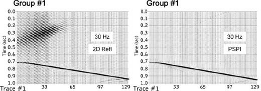
Comparison of zero offset sections of a single dipping bed obtained by 2-D reflectivity method and PSPI. The former method produces strong numerical noise (see text).
2 Theory
2.1 Extension of reflectivity method from 1-D to 2-D
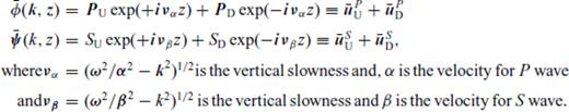
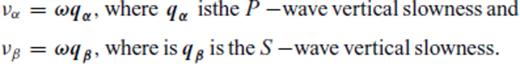
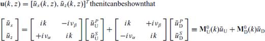
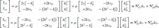
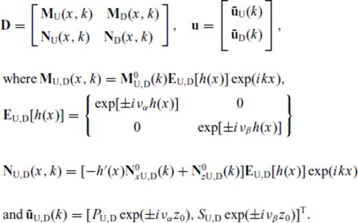
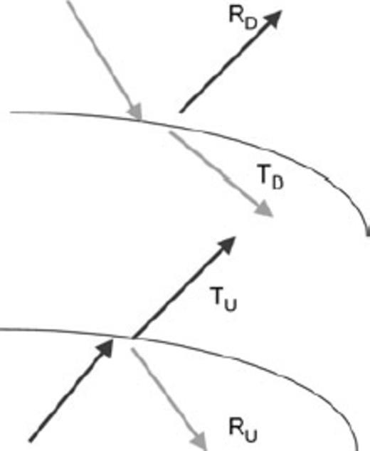
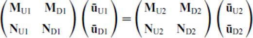
The 1-D reflectivity method is exact for the case where media parameters vary only in one (vertical) direction or equivalently, all interfaces between layers are horizontal. For each frequency ω and ray-parameter p, the angle dependent upward and downward looking reflection and transmission coefficients are computed at each interface from conditions of continuity of displacement u and normal stress τ across an interface between, say, regions 1 and 2 (Fig. 2a). These coefficients and the propagation within a homogeneous layer form the basis for the four fundamental ‘reflectivity’ matrices RD(p), RU(p), TD(p), TU(p) that represent the exact cumulative response of a stack of horizontal layers in terms of reflection and transmission in the frequency-wavenumber (or equivalently frequency-horizontal slowness p) domain. The response of different target zones can be computed separately and combined with those of the overburden regions to obtain the complete seismogram. Among the remarkable features of the method are propagation mode conversion and the natural inclusion of interbed multiples of all orders.
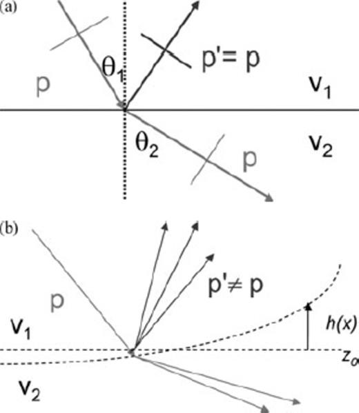
(a) The horizontal slowness is conserved for an incident ray after reflection from a flat interface between region 1 and 2. (b) An incident ray with slowness p is scattered into those with different p′ after reflection off a general curved interface which may be considered as a conglomeration of point scatterers.
Extension of the reflectivity method to two dimensions, where the velocities and densities are allowed to vary laterally as well, is non-trivial. In this paper, we restrict the lateral heterogeneity to the case of homogeneous layers separated by irregular or curved interfaces, which do not cross each other. Lateral media variations within a layer cannot be easily taken into account in a reflectivity-type formalism because the concept of an interface is inherent in it except using the concepts of pseudo-differential operators and Fourier Integral operators (McCoy et al. 1986).


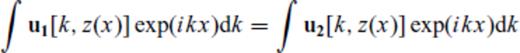
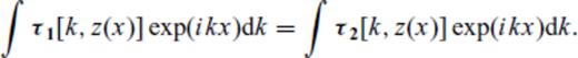

The solution of these simultaneous equations yields the familiar ‘up/down’ looking reflection and transmission coefficients RD(p), RU(p), TD(p), TU(p).
Across a flat surface, the horizontal slowness p or wavenumber k is conserved according to Snell's law. However, across an irregular interface, an incident ray with a particular p is scattered into different p′ (Fig. 2b). This is mathematically equivalent to Fourier transforming the dependence of z on x to the scattered set of p′ or k′. Now the coefficients RD(p), RU(p), TD(p), TU(p) become functions of both p and p′.

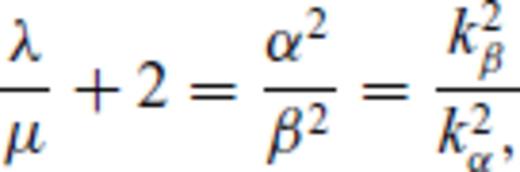
Now let us consider an irregular interface z(x) = z0 + h(x) (Fig. 2b) between layers 1 and 2 with the underlying assumption h(x) ≪ z0 (i.e. undulations of the interfaces are small and the latter do not cross each other).
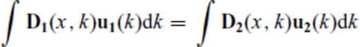

Note that for h(x) = 0 (flat interface), these matrices are diagonal. For the SH and for the acoustic cases, dimension of the matrices is 2N while for P−SV case it is 4N.

Generalized definition of reflection and transmission coefficient matrices for a general curved interface.
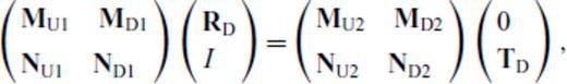
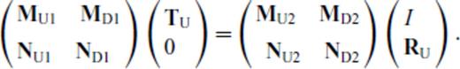
Eqs (4) and (5) are finally solved for RD, RU, TD, TU which are now functions of both p and p′ in terms of the matrices M(p, p′) and N(p,p′) defined above by the ‘invariant embedding approach’ of Koketsu et al. (1991). As already discussed, all these matrices are diagonal for a flat interface. However, for the next least complex case of an interface with a single dip, the matrices can be analytically shown to have non-zero elements along shifted diagonals. Inversion of these highly rank-deficient matrices gives rise to numerical artefacts—as a matter of fact, inversion becomes much less noisy for varying and conflicting slopes when the matrices become dense—for example, in a basin-like structure that has been quoted widely in related literature.
 we have
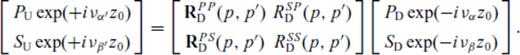

Koketsu et al. (1991) derived explicit expressions for Q(p, p′), where Q stands for RD, RU, TD, TU which may be shown to reduce to Q(p) for a flat interface.
At this stage we differ from the approach of Koketsu et al. (1991) in that we examine the seismograms in the coupled slowness domain which offers an easy interpretation that is analogous to 1-D τ-p interpretation for modelling, multiple attenuation and migration. In this procedure, we produce three kinds of seismograms, each of which has tangible correspondence with those obtained for the 1-D case.
2.2 General methodology for generation of seismograms in slowness and spatial coordinates


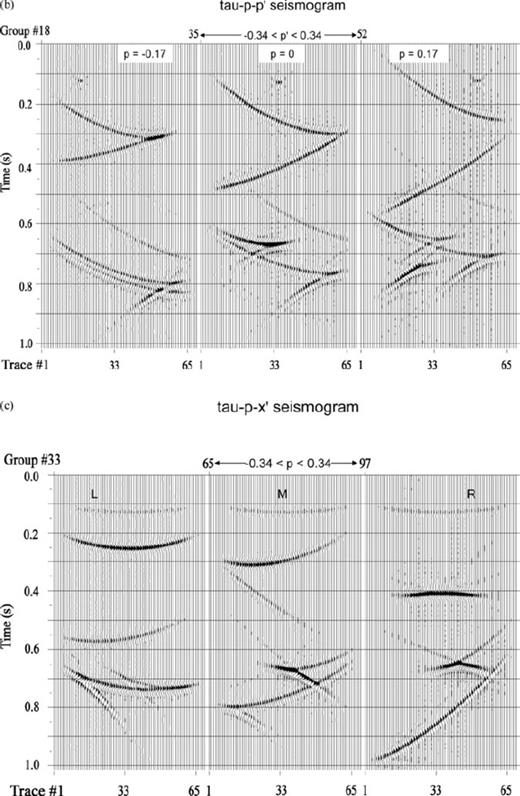
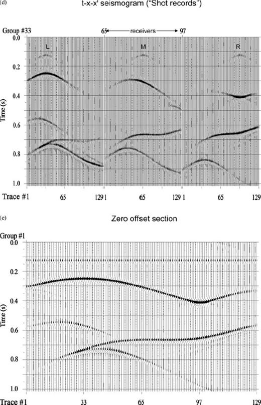
![(a) Single dipping bed model overlain by a flat interface. (b) Corresponding τ-p-p′ seismogram: Note that we have non-zero contribution for p = p′ from flat interface while the response for the dipping reflector is shifted to p ≠ p′. (c) Corresponding τ-p−x′ seismogram: for three different receiver locations [marked as L, M and R in (a)], note that the τ-p curve is elliptical for the top horizontal reflector while that for the lower reflector is a shifted and tilted ellipse. (d) Shot records at points L, M, R along the shot profile (see text): apex of the reflection hyperbolas coincide with the shot location for the top reflector whereas the hyperbolas corresponding to the bottom reflector is shifted. (e) Zero offset section for the model shown in (a).](https://oup.silverchair-cdn.com/oup/backfile/Content_public/Journal/gji/178/2/10.1111/j.1365-246X.2009.04172.x/3/m_178-2-792-fig004.jpeg?Expires=1716434288&Signature=kNHvqbQYyh6kwGV9uAMwZcywhLYwLd1rXmzimhvW0fpetrXIFKP3xcf9vVRnI8BH5Milx2cfEaey0XXe99TCJkSt81mw9VhHEDCtqQlzPi3BN304T3xFJ3wBuA~ZqP-qjvgZge8iuII2Ig3NV7yicYwQry55kspvh-ZANe75-UaVUl7encyRPAKaMGUGL0ch~SoMpAXCmkyPOzCrkKUQZQYM0I72JsJVYBTkvBiSK0MyuJgJM2tlQqyQ2iUvjVwsgBuDBcU0laHErRp4-Aq7mgdQX0QjTq93WkU0Bpv-FbIO3aFzs69VgXebCpGCZPBHTJBJBuZYUXFZusDkUExNXQ__&Key-Pair-Id=APKAIE5G5CRDK6RD3PGA)
![(a) Single dipping bed model overlain by a flat interface. (b) Corresponding τ-p-p′ seismogram: Note that we have non-zero contribution for p = p′ from flat interface while the response for the dipping reflector is shifted to p ≠ p′. (c) Corresponding τ-p−x′ seismogram: for three different receiver locations [marked as L, M and R in (a)], note that the τ-p curve is elliptical for the top horizontal reflector while that for the lower reflector is a shifted and tilted ellipse. (d) Shot records at points L, M, R along the shot profile (see text): apex of the reflection hyperbolas coincide with the shot location for the top reflector whereas the hyperbolas corresponding to the bottom reflector is shifted. (e) Zero offset section for the model shown in (a).](https://oup.silverchair-cdn.com/oup/backfile/Content_public/Journal/gji/178/2/10.1111/j.1365-246X.2009.04172.x/3/m_178-2-792-fig005.jpeg?Expires=1716434288&Signature=25eOaOkFPAp5dU3CQgiRmEPBVaApG0M-WlcW~dPZYSXFgcx1QEUqP0XJCeGB-Yzf0EJmbsfuZwbmAbZsEYUm8bsXB3KsD2~1lHcsJdJCd04UHTkdiru6vVlFb0hwD-cLRTtTe3rDstB3UbNwb0tYvHg2Rp2Aj2NDcnZzMh7V22T7RtvJG-0RQjpn48qAGTtBji8JhOTFE5Y0ckn3EJ-cbPkjXVFk3UjaUbYvDq4VrYwqQWlqMDIkHVjhpUOJDQuGD4TG-y-LPCuEa-rADtzcxvcX-VNH50u9o4VjcXPjyXrNLYBKqKst0EIdvFmc-SWof28GIu03dfKvHTA9Vfz1-g__&Key-Pair-Id=APKAIE5G5CRDK6RD3PGA)
![(a) Single dipping bed model overlain by a flat interface. (b) Corresponding τ-p-p′ seismogram: Note that we have non-zero contribution for p = p′ from flat interface while the response for the dipping reflector is shifted to p ≠ p′. (c) Corresponding τ-p−x′ seismogram: for three different receiver locations [marked as L, M and R in (a)], note that the τ-p curve is elliptical for the top horizontal reflector while that for the lower reflector is a shifted and tilted ellipse. (d) Shot records at points L, M, R along the shot profile (see text): apex of the reflection hyperbolas coincide with the shot location for the top reflector whereas the hyperbolas corresponding to the bottom reflector is shifted. (e) Zero offset section for the model shown in (a).](https://oup.silverchair-cdn.com/oup/backfile/Content_public/Journal/gji/178/2/10.1111/j.1365-246X.2009.04172.x/3/m_178-2-792-fig006.jpeg?Expires=1716434288&Signature=hUJJrUe-MfQhPZMz5cjCPxzupv0B4BadqIB7hc34ZDYzpP~yoZ8uiPsKoJQSWed~gIY6sZOKQBbEkhbu24bDewfbKx1d0cTWwZ6JAaBqpLfvoQdZhatSVdvpbX9thRsgIuBCFgy5aa3YrNee5ny8TP6lZLgETDN8YUsGgwxIgZyZ0RIF3NNh2II~vxzVbPG89ztRQjydEtJP1Pgk7NbgYIcvFeBHOuQvmfP9mKF7MWnkyW8I~TjMhNUvbMyVmy4cY-rBRlWN3QIZm7w2Xd63NC63sLts5n92IO9D0bi2QgUpamfVFdisUYWMD90RSGWCsxpxU0XsiFLGDn~RGZ0~ew__&Key-Pair-Id=APKAIE5G5CRDK6RD3PGA)
(a) Single dipping bed model overlain by a flat interface. (b) Corresponding τ-p-p′ seismogram: Note that we have non-zero contribution for p = p′ from flat interface while the response for the dipping reflector is shifted to p ≠ p′. (c) Corresponding τ-p−x′ seismogram: for three different receiver locations [marked as L, M and R in (a)], note that the τ-p curve is elliptical for the top horizontal reflector while that for the lower reflector is a shifted and tilted ellipse. (d) Shot records at points L, M, R along the shot profile (see text): apex of the reflection hyperbolas coincide with the shot location for the top reflector whereas the hyperbolas corresponding to the bottom reflector is shifted. (e) Zero offset section for the model shown in (a).
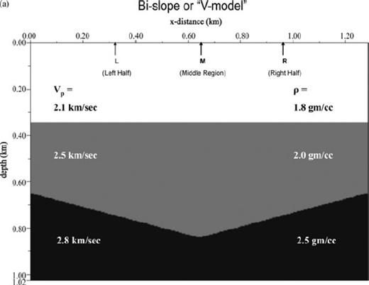
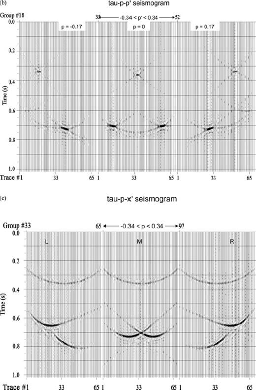
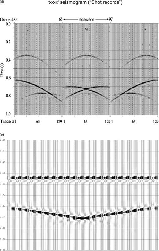
(a) The ‘V-model’—beds dipping in opposite directions. (b) Corresponding τ-p-p′ seismogram: Similar to Fig. 6(b) except that the response for the symmetrically dipping bottom reflector is shifted to both sides of incident p to scattered p′≠ p. (c) Corresponding τ-p−x′ seismogram: the distorted elliptical τ-p curves corresponding to the lower reflector cross each other symmetrically for location at the middle of the profile and asymmetrically for receivers towards the edges. (d) Shot records at points L, M, R along the shot profile for the ‘V-model’. The shifted reflection hyperbolas cross each other (corresponding to the opposite slopes of the lower reflector) at different x-locations and time values depending on the shot positions. (e) Zero offset section for the model shown in (a): the crossing of two branches corresponding to the conflicting slopes in the model is clearly seen.
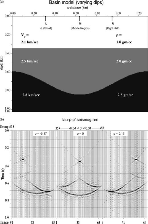
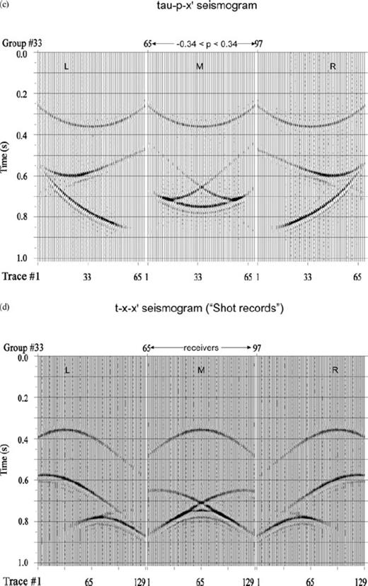
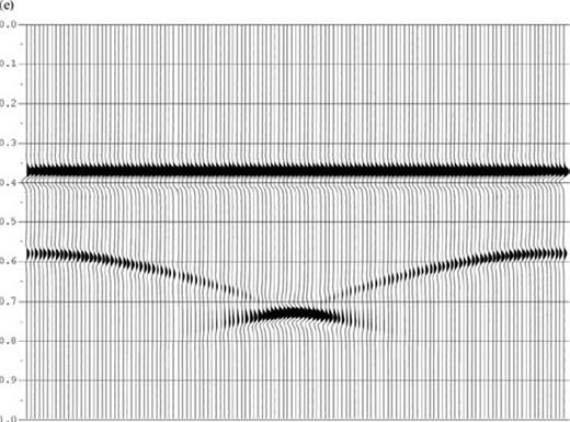
(a) Basin model overlain by a flat bed. (b) Corresponding τ-p-p′ seismogram: comparing with Fig. 7(b), note that a particular p is scattered to a continuous range of p′s whose delay times cross each other due to a whole range of equal and opposite slopes present in the basin structure in place of a single pair of such slopes in the V-model. (c) Corresponding τ-p−x′ seismogram: the features described in (b) is reflected in the τ-p seismograms at three locations L, M and R marked on the model. (d) Shot records at points L, M, R along the shot profile (see text) show the expected ‘triplication’ in the arrival times corresponding to the basin shape of the lower interface. (e) Familiar ‘bow-tie’ zero offset section for the basin model shown in (a).
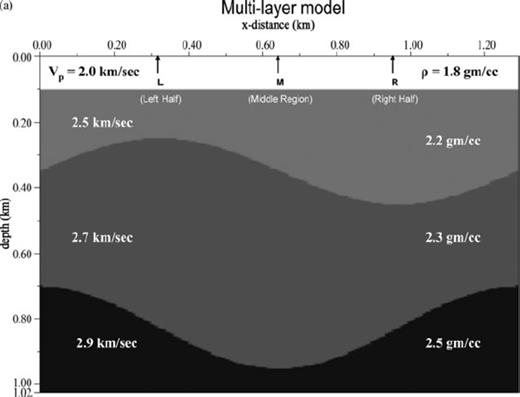
(a) A multi-irregular layer model—a ‘sine wave’ shaped interface followed by a basin structure below a top flat layer. (b) τ-p-p′ seismogram for the multilayer model showing different branches corresponding to successive interfaces. (c) Corresponding τ-p−x′ seismogram for the multilayer model. (d) Shot records at points L, M, R along the shot profile (see text) show varied natures of ‘triplication’ in the arrival times corresponding to the ‘sine wave’ and basin shapes of the lower interfaces. (e) The multilayer zero offset section shows small ‘triplication’ (just below the top flat reflector) due to the trough part of the upper ‘sine wave’ structure and a bow-tie due to the basin shape below but modulated by the sinusoidal interface above it.
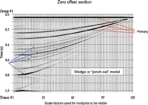
Zero offset section showing generation of multiples in a ‘wedge-type’ model (in which two curved layers merge against a horizontal interface) by PSPI based reflectivity method. Note the opposite polarity of the first order interbed multiples. Scale factor has been used for the multiples to be visible.
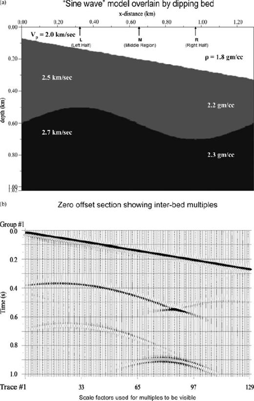
(a) A model with ‘sine wave’ structure overlain by a dipping bed. (b) The zero offset section for the above model demonstrates: (i) transmission through a non-horizontal interface; (ii) tilted bow-tie effect due to the dipping reflector above and (iii) the first-order interbed multiple.
2.3 Kirchhoff-Helmholtz formulation
 . In region 1 containing the ‘image’ or ‘virtual’ source
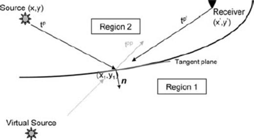
Source, receiver and irregular interface configuration for Kirchhoff-Helmholtz formulation of Sen & Frazer (1991).

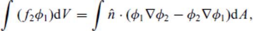
It may be noted that in 2-D, the ‘surface integral’ on the right hand side becomes a ‘line integral’ along the irregular interface.
Assuming homogeneous layers, Sen & Frazer (1991) used ray-parameter expansions of the general source and receiver wavefields resulting in an interaction between plane waves only at each point at the surface of integration—a generalization called multifold phase space path integral (PSPI) by them. It results in the following equation:

Let us now compare eqs (6) and (11). In the former (2-D reflectivity method), the reflected wavefield including the ‘phase term’ is given in the ω-p-p′ domain with the reflection coefficient RD(p, p′) calculated explicitly in terms of undulations h(x) over some ‘mean’ horizontal depth z0 and its derivative h′(x). The latter equation (KH integral formulation) gives the same field directly in the ω-x-x′ domain as a three-fold integral over p, p′ and all positions x1 along the interface with the reflection coefficient put as in Aki-Richards formulation incorporating local slope in the ‘tangent plane approximation’; the variation in z1(x1) is also included in the phase term.
In view of the previously discussed matrix inversion problem in 2-D reflectivity approach, we transform the asymptotic but simpler PSPI formulation in ω-x-x′ domain to ω-p-p′ domain and show its correspondence to the other method. Once the equivalence is established, one may use the cheaper and stable PSPI method and utilize, at the same time, the recursive property of 2-D reflectivity formulation to generate ω-p-p′ seismograms which are then transformed successively to τ-p−x′ (τ-p seismograms at all receiver positions), t−x−x′ (shot records at all locations along a profile) and zero-offset sections. Thus the combination of PSPI in ω-p-p′ domain and the technique of successive transformations from p to x domain—a natural extension of seismogram generation in 1-D—provide a cheap and viable methodology of seismogram synthesis in presence of lateral velocity variations.
3 Correspondence Between Reflectivity Approach (Koketsu, Kennett) and Pspi (Sen & Frazer 1991)
 we have

L being the spatial extent of the model.

 (see Fig. 5)
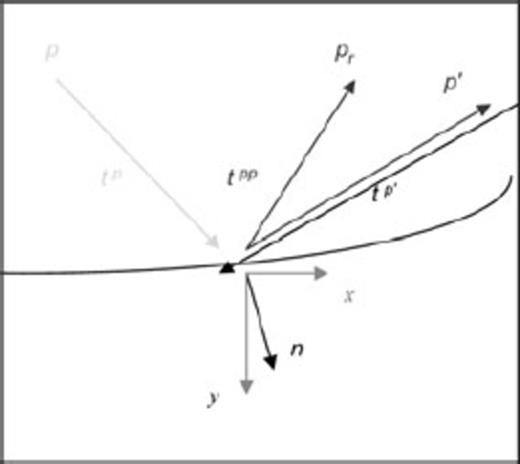
Diagram for showing the correspondence between slowness components and ray directions in 2-D reflectivity and PSPI methodologies.
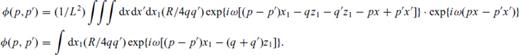
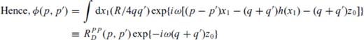
For a flat interface [h(x1)= 0], the ω-p-p′ seismogram is given by φ(p, p′) = (RPPD)δ(p−p′) exp{−iω(q + q′)z0}.
It may be noted that eq.(15) is very similar to eq.(6) in 2-D reflectivity approach (with the notation for vertical slowness being changed from ν to q). The difference, however, is that both the undulation h(x1) and its derivative enter explicitly in the calculation of RPPD(p, p′) in eq. (6), whereas in eq. (15), only the depth variation h(x1) gets integrated over x1 in the ‘phase term’ to give an equivalent effect. The two approaches converge in the limiting case of a flat interface, that is, h(x) = 0.
4 Examples
In this section, we show synthetic seismograms for several models, from the simplest to increasing degrees of complexity in terms of the ‘curvedness’ of the interfaces and their numbers. The corresponding τ-p-p′, τ-p−x′ and t−x-x′ responses at the surface (z = 0) are shown to demonstrate the efficacy of the approach adopted in this paper which may be termed as ‘PSPI based reflectivity’. The models are chosen in such a way that first, the responses of the simple ones can be interpreted easily and compared to the expected τ-p and t−x domain results known from independent methods like the Kirchhoff ray-based modelling. The methodology is then applied to more complicated models with a variety of irregular interfaces. The stability of the procedure is established (confirmed) by propagation down a number of layers and the generation of interbed multiples.
Figs 6(a)–(e) to 8(a)–(e) depict three-layer, two-interface models and their responses (primaries only) in which the first interface is taken as flat to have the simplest transmission down to the non-flat interface below [a single dipping bed in Fig. 6a, a symmetric cross-dipping bed (the ‘V-model’) in Fig. 7a and a basin structure in Fig. 8a]. The case in which both the interfaces are curved is shown (as zero offset section with multiples) in Fig. 11 while Figs 9(a)–(e) show a three-interface model and its primary-only response. All the models have horizontal extent of 1.28 km and vertical extent ∼1 km. In panels 6–9(c) and 6–9(d), the responses correspond to surface locations L, M and R marked on the models at x = 0.32 km (middle of left-side half), x = 0.64 km (middle point) and x = 0.96 km (middle of right-side half) respectively. In Figs 6–8, velocities of layers 1, 2 and 3 are v1 = 2.1, v2 = 2.5, v3 = 2.8 in km s−1 and the corresponding densities are ρ1 = 1.8, ρ2 = 2.0, ρ3 = 2.5 in g cc−1, respectively. The τ-p-p′ seismograms, depicted explicitly in this work, vividly show the expected p-values of reflected or scattered rays off an interface corresponding to a particular incident direction. The p-values (in s km−1) range from −0.34 to +0.34 at an interval of 0.01 in all the figures.
For a single interface dipping from left- to right-hand side, the scattered p-values shift to the more positive directions—rays with p = 0 shift to p′ = 0.17 and rays with p = −0.17 get scattered to p′ = 0 (Fig. 6b) whereas they scatter to opposite directions for beds with conflicting mono-slopes (Fig. 7b). In the case of the basin-like interface having a range of slopes of opposite sign, the scattered p′-values form a continuously distributed self-crossing ‘structure’ (Fig. 8b).
After a first transformation from the slowness domain to space domain, these features get reflected in the τ-p−x′ plots (τ-p seismograms at different locations along a profile shown in Figs 6–8c). The familiar symmetric ellipses correspond to flat interfaces; the rotated and distorted ellipses result from reflections from slopes while the V-model and synclinal bedding give rise to intersecting ellipses with different orientations corresponding to different incident rays. The space-domain one-shot-multireceiver gathers (obtained by an additional transform from p to x domain) having the shape of hyperbolas corresponding to flat interface, tilted hyperbolas for dipping beds and hyperbolas with ‘triplicated’ traveltimes for synclinal structure are shown in Figs 6–8(d). The zero-offset sections displayed in Figs 6–8(e) conform to known results obtained from the Kirchhoff ray-based modelling. Figs 6–9(c) show the τ-p seismogram at locations marked L, M and R along the profile and Figs 6–9(d) are the shot gathers with shot at these locations and receivers placed all along the profile at an interval of 10 m.
A more complicated multi(curved) layer model (a ‘sine wave’ shaped interface followed by a basin structure below a top flat layer) and its responses (Figs 9a-e) are included to show the stability of the recursion of reflection and transmission matrices corresponding to propagation of wave down a stack of irregular layers. Note the indication of triplication below the trough part of the sine wave interface and the pronounced triplication of arrival times corresponding to the basinal structure that is tilted due to the presence of sinusoidal interface above it in the t-x-x′ and zero-offset seismograms. In Figs 6–9, only primary reflections are shown although the method is equipped to generate interbed multiples which are included in the next two figures. Fig. 10 depicts only the zero-offset section (to avoid repetition of similar figures) showing interbed multiples along with the primaries of a wedge or pinch-out model. Note the opposite polarity of the multiple arrivals from those of the primaries. Apart from the generation of interbed multiples for a multicurved-layer model, this model demonstrates that the PSPI based reflectivity method is capable of producing reasonable results even when the interfaces merge with each other as in this simple wedge model. Figs 11(a) and (b) show the model and its zero offset section (with first order multiple) in which the first interface is also not horizontal. Note the tilting of the basin structure related triplication of arrival times due to the sloping interface above. This example further establishes the validity of proper reflection and transmission through a set of arbitrarily curved layers in this methodology that does not require the first interface to be horizontal.
5 Discussions and Conclusion
We have employed a viable combination of exact and asymptotic methods to generate noise-free seismograms in the coupled slowness (τ-p-p′), common shot with varying receiver slowness (τ-p−x′) and familiar shot-receiver (t−x-x′) domains. Explicit responses in all three domains for several models of varying complexity have been demonstrated for the first time. This PSPI based approach has clear advantage over the rigorous 2-D reflectivity method in generating noise-free seismograms. It eliminates the unwanted numerical artefacts that are unavoidable in the latter approach due to inversion of several rank-deficient matrices. The comparison is clearly shown in Fig. 1. The only noise in the PSPI approach is due to edge effects and the replacement of slowness and spatial integrals by sum over finite number of discrete variables in the numerical implementation. The edge effects are largely taken care of by suitable tapering. Costwise, the time taken by this semi-analytic approach is a few orders of magnitude lower compared to that of finite difference calculation for a typical 2-D model. The added advantage is that all three types of seismograms are produced in a cascaded process in which finally all shot records along a profile are generated simultaneously. This saves a lot of computer time.
It is emphasized once again that the case of laterally varying media considered here is restricted to homogeneous layers separated by irregular interfaces, which do not cross each other. Efforts are under way to generate similar set of responses for a general heterogeneous medium.
Acknowledgments
The authors wish to thank Shell and Jackson School of Geosciences for their support for this work. We thank two anonymous reviewers and the associate editor for many helpful comments.
References
