Full waveform tomography for lithospheric imaging: results from a blind test in a realistic crustal model

Summary

Introduction

A typical approach taken to overcome limitations in resolution and robustness to noise of surface seismic surveys has been to increase the spatial instrument sampling of an experiment. Active source, wide-angle surveys designed to image the upper portions of the lithosphere may benefit from increased sampling densities in either the shot or receiver domains. As the number of broadband instruments available for wide-angle seismic experiments increases, denser sampling is possible, and improved images of the subsurface become attainable. Although the methods and design of controlled-source seismic acquisition programs for imaging of the lithosphere may be varied, the velocity estimation strategy applied to the recorded data has typically been limited to traveltime tomography (Rawlinson & Sambridge 2003). Traveltime tomography, based upon ray tracing or the direct solution of the eikonal equation (Vidale 1990), can use either reflection or refraction traveltimes, or a combination of both, to invert for a velocity model of the subsurface.

A common approach to traveltime tomography is to use a finely gridded parametrization to seek a smooth or minimum structure model using only one or two prominent data phases and little a priori information (e.g. Scales 1990; Zelt & Barton 1998). Alternative methods can incorporate geologically reasonable interfaces or other subjective information. Zelt (2003) recently presented an assessment of traveltime tomography methods. They advocated a hybrid approach, deriving preferred models based upon complementary features from different models and a priori geologic knowledge. Even with this hybrid approach, velocity models obtained by traveltime tomography are generally resolution limited to the first Fresnel zone (Williamson 1991; Williamson & Worthington 1993; Schuster 1996; Dahlen 2004); reflection times may allow somewhat better localization in the case of interfaces (e.g. McCaughey & Singh 1997).

The seismic waveform contains much more information about the medium of propagation than is typically used in traveltime tomography. The full information content of the seismic waveform can potentially be accessed by waveform inversion methods (Devaney 1984; Tarantola 1984). Waveform inversion may be implemented in time–space (Tarantola 1986; Mora 1987; Shipp & Singh 2002) and frequency-space domains (Pratt 1990; Liao & McMechan 1996). Surface-wave tomography is a common form of waveform inversion, and is generally applied on regional or global scales (Nolet 1987). Traditional teleseismic crustal-imaging methods, where naturally occurring earthquakes are used as sources, have recently become capable of recovering higher-resolution images of the crust by combining the methods of receiver functions and the inversion of scattered body-wave coda (Rondenay 2001; Bostock 2002).

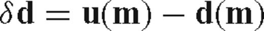
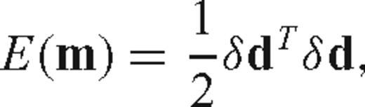
In waveform inversion, a ‘best fit’ model is recovered by iteratively minimizing the misfit between the real, ‘observed’ waveform data, and the synthetic, or ‘calculated’ waveform data from forward modelling. Due to the high computational cost of calculating the synthetic data, the non-linear inverse problem is usually solved by local methods (Tarantola 1984; Pica 1990; Sun & McMechan 1992). A detailed review of many waveform inversion methods is provided by Pratt (1998). Waveform inversion of complicated, 2-D earth models, such as the Marmousi model (Versteeg 1994), succeeded when a multiscale approach was used, starting with a sub-sampled, low-frequency version of the input data and iteratively increasing the scale of the problem as the inversion progressed (Bunks 1995; Sirgue & Pratt 2004). A multiscale approach has also been applied to 2-D waveform inversion of real, wide-angle data recorded on 12 km marine streamers, though computational restrictions allowed only a small subset of the data to be analysed (Shipp & Singh 2002).

We use the term waveform tomography to describe a process which begins by using traveltime tomography methods to obtain a starting model near the global minimum of the non-linear inverse problem, followed by application of waveform inversion to the earlier arrivals of the data. The process of traveltime tomography followed by frequency-domain waveform inversion has been thoroughly reviewed by Dessa & Pascal (2003), and was applied to real seismic data by both Brittan (1997) and Dessa (2004). The high computational costs typically associated with waveform tomography are mitigated by implementation in the frequency-domain (Pratt & Worthington 1990). For a simple crustal model, Pratt (1996) generated a synthetic seismic data set and compared the results of traveltime and waveform tomography with wide-angle seismic data. The results, although preliminary, demonstrated that waveform tomography could provide images of a crustal velocity model at a resolution higher than those attainable by traveltime tomography alone, if the acquisition geometry was designed with densely spaced sources and receivers.

Solving the waveform inverse problem successfully is critically dependent upon the accuracy of the starting model and the minimum inversion frequency, since the highly non-linear nature of the problem can cause the solution to converge to a local rather than a global minimum (e.g. Mora 1987). In the absence of any direct knowledge of the subsurface, the efficacy of the waveform tomography approach can only be evaluated by comparison of the original data with the data predicted by the best fit model, or by an analysis of the geological feasibility of the model. Frequency-domain waveform tomography has been successfully applied to real, wide-angle data acquired across the edge of the Chicxulub impact structure (Brittan 1997), in the axial zone of the southern Apennines fold and thrust belt (Operto 2004; Ravaut 2004), and to OBS data over the Nankai trough, a subduction zone in the Japanese arc (Dessa 2004). In these real data examples, complex geological structures were imaged with waveform tomography at a resolution unattainable by the results from traveltime tomography. In addition, the results from the southern Apennines fold and thrust belt were verified directly through a comparison with borehole data.

In this paper we describe a blind experiment with third-party, synthetic, realistic (though relatively noise free), 2-D, viscoelastic, densely sampled, crustal-scale, large-offset, wide-angle, seismic data. Our results demonstrate that such data can be successfully inverted to obtain high-resolution velocity structure, using a strategy combining traveltime and ‘full’, 2-D, acoustic waveform tomography. The term ‘full’ waveform tomography is used to indicate that a complete sampling of the useful bandwidth of the data is used in the inversion. We employed a multiscale strategy, applying waveform tomography in six different stages, with each subsequent stage resolving increasingly higher spatial-wavelength-scale features within the unknown velocity model. Our results were generated without any knowledge of the original, ‘true’ model. When the true velocity model was revealed, it was evident that we had accurately imaged the velocity model with both vertical and horizontal resolutions of approximately 1 km within the central portion of the model.

Following the blind test and the application of full waveform tomography, in a further investigation, the ‘efficient’ waveform tomography strategy of Sirgue & Pratt (2004) was used to achieve results nearly equivalent to those obtained from full waveform tomography by employing a carefully selected subset of input frequencies, at a fraction of the computational cost. These results are fully documented in an accompanying paper, (Brenders & Pratt 2006, submitted manuscript), hereafter referred to as Paper II, in which we further investigate the spatial sampling requirements, and the minimum starting frequency, for waveform tomography of wide-angle seismic data.

In the first part of this paper, we present a short summary of the theory of waveform tomography. The second part of this paper describes the CCSS data set and model in detail. In the third part of this paper, we present the strategy for the successful application of 2-D, frequency-domain acoustic full waveform tomography to realistic data generated in an unknown velocity model in a blind test. Our strategy for successful waveform tomography consists of the following major steps:

• (i)

  Generation of an accurate starting velocity model by first arrival traveltime tomography, to mitigate the non-linearity of the inverse problem and avoid convergence to a local minimum;

• (ii)

  Forward modelling of synthetic waveforms for qualitative assessment of the ability of the starting model to match waveforms to within a half-cycle and correctly predict the acoustic amplitude-versus-offset response;

• (iii)

  Preconditioning and quality control of the input data to choose the lowest viable frequency present in the data, improve the chances for accurate inversion with the acoustic wave equation by removal of dominant elastic phase and amplitude information, and sub-sampling input gathers to remove traces with low signal-to-noise ratios;

• (iv)

  Sequential, frequency-domain waveform inversion, proceeding from low to high frequencies, applying preconditioning operators to both data and residuals in order to improve convergence;

• (v)

  Forward modelling within the final velocity model to compare ‘synthetic’ and ‘observed’ data waveforms.

The presentation of this strategy is followed by a discussion of our results.

The mathematical symbols used in this paper are presented in Table 1.

Table 1

Open in new tabDownload slide

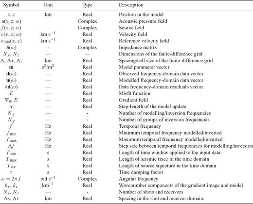
List of mathematical symbols used in this paper.

Theory

The excessive computational cost of multisource time domain waveform tomography was significantly reduced by implementation of forward modelling in the frequency domain with the acoustic wave equation (Pratt & Worthington 1990). Although waveform tomography with the elastic wave equation is possible (Pratt 1990), this approach has not been as fully developed as acoustic methods. In this paper, we consider wave propagation as described by the isotropic, 2-D, visco-acoustic wave equation,

1

where ρ(x, z) is the density, κ(x, z) is the bulk modulus, ω is the angular frequency, u(x, z; ω) is the pressure field and f(x, z; ω) is the source term. Attenuation is implemented by defining velocity to be a complex-valued quantity,

2

where c_Re(x, z; ω) is the real component of the velocity, the imaginary component is

3

Q is the Quality factor, and both c_Re and c_Im may vary arbitrarily with frequency.

In discrete form on a two-dimensional (2-D) grid, following the work of Pratt (1998), the resulting numerical system of equations corresponding to eq. (1) can be written as

4

where the complex-valued impedance matrix, S(m; ω), approximates the physics of the wave equation operator in discrete form. The source wavefield, f(ω), and pressure wavefield, u(m; ω), are defined in two dimensions and are stored for each frequency as vectors with dimensions N_x×N_z, where N_x and N_z define the dimensions of a finite-difference grid with a regular node spacing of Δ, where Δ=Δx=Δz. The impedance matrix depends explicitly on the (2-D) acoustic model parameters, m(x, z), representing density and velocity, also defined on the same 2-D grid. The pressure field, u(m; ω), can thus be calculated by solving this system of linear equations. Solutions for a large number of source terms can be obtained by, for example, LU factorization of the impedance matrix, followed by forward and back substitutions. The LU factorization is efficiently carried out by the nested dissection method of George & Liu (1981). Discretization of the acoustic wave equation also allows the highly accurate, mixed-grid finite-difference approach of Jo (1996) and Štekl & Pratt (1998) to be used. For a model defined on a regular finite-difference grid, absorbing boundary conditions can be implemented at the edges of the model using 45 degree one-way propagators, adapted from the method of Clayton & Engquist (1977). To effectively prevent reflections and diffractions at the corners of the model, where the 45 degree one-way propagators are less effective, additional boundary absorption can be introduced by assigning gridpoints a finite Q value.

The forward problem of eq. (4) allows us to predict the seismic data, u(m; ω), for a given source-receiver configuration, and for a given set of parameters, m, defined for each value of x and z on the 2-D grid. To solve the waveform tomography problem, we need to find a set of model parameters, m, that allow us to calculate synthetic wavefields, u, which match our ‘real’ seismic data, d, to the greatest degree possible. Defining the residual error as

5

(and dropping the explicit dependence on ω), the difference between the wavefield calculated in a given model, u(m), and the observed wavefield, d(m), m must be found such that δd(m) is a minimum. Thus, we seek the solution to the inverse problem, which minimizes the sum of the squared residuals,

6

where E(m) is the l₂ norm misfit (or objective) function, and δd^T represents the conjugate transpose of the residual error.

We solve the non-linear waveform inversion problem by the gradient method: For a given starting model, an initial forward-modelling step is made, using the methods described above, in order to calculate the data residuals given in eq. (5). New models may be iteratively calculated by updating m with

7

where k is the iteration number, α is the scalar size of the model update, and ∇_mE is the gradient of the misfit function, taken with respect to the model parameters. The model perturbations, or the values by which the model is updated, are calculated by multiplication of the gradient of the objective function with a step length α, which must be repeatedly calculated. Mathematically, the gradient may be computed as a multiplication of the frequency-domain forward-modelled pressure wavefield with the backward propagation of the residuals. This is also known as the ‘virtual source’ method, the details of which are found in Pratt (1998). Hence, only two forward problems need to be solved per frequency: the wavefield for a source located at each shot position, and the backward propagated residual wavefield ‘composite’ source. Since the computation of the step length, α, also requires the solution of at least one more forward problem, a minimum of three forward problems need to be solved for each iteration of non-linear waveform inversion. The conjugate gradient method is easily applied to improve convergence of the gradient method.

Waveform tomography with the acoustic wave-equation requires a source function, f(ω), as in eq. (4). Pratt (1999) estimates the unknown source signature by a complex-valued scalar, s,

8

equal to the cross-correlation of the forward-modelled wavefield from modelling in the current velocity model with the conjugate of the observed wavefield, divided by the auto-correlation of the forward-modelled wavefield (Pratt 1999). This method converges in one iteration and provides a good estimate for both the amplitude and phase of the true source signature provided the velocity the model is at least approximately correct.

Waveform Tomography: A Blind Test

A realistic crustal model: The 2003 CCSS data set

In 2003, a synthetic, long-offset synthetic seismic data set was made available in preparation for a workshop on modelling, inversion and imaging of controlled-source seismic data (Zelt 2005). The data were generated in a realistic, viscoelastic, crustal geology model that was kept unknown from participants prior to the workshop in order to facilitate a blind test of imaging methods. The test was administered by Colin Zelt and John Hole for the 12th International Workshop of the Working Group on Seismic Imaging of the Lithosphere (WGSIL), formerly known as the Commission on Controlled Source Seismology (CCSS, a division of IASPEI).

The CCSS model represented a section of continental lithosphere 250 km in length and 40 km in depth. It was specified on a grid of 5557 × 890 nodes, using a 45 m node spacing, by values of three primary physical parameters at each node: ρ, λ, and μ. The P-wave velocity model was generated by using the equation

9

where v is the velocity of a given node, λ is the Lamé constant, μ is the shear modulus, ρ is the density, and i and j indicate the position of the node within the grid. The true CCSS model was only revealed to all participants on the final day of the CCSS workshop, following the presentation of the tomographic results given in this paper, but is presented here in Fig. 1(a).

Figure 1

Open in new tabDownload slide

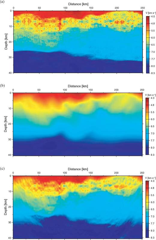
P-wave velocity models for (a) the true model used to compute the synthetic data, (b) the starting model for subsequent waveform tomography using all 141 729 hand picked first arrivals, and (c) the final model derived from waveform tomography. The blind test recovered a spatial resolution on the order of 1 km within the central and near-surface portions of the model.

As described by Zelt (2004), the Poisson's ratio, σ, defines six distinct regions with the model, each characteristic of a specific geological feature: an upper layer of sediments (σ= 0.200), the upper crust (σ= 0.267), a low-velocity zone within the upper crust (σ= 0.317), the lower crust (σ= 0.255), the crust–mantle transition zone or Moho (σ= 0.246), and the upper mantle (σ= 0.242). Density values within the model range from 2.38 g cm⁻³ to 3.48 g cm⁻³, and the P-wave velocities range from 4.0 to 8.3 km s⁻¹. A low-velocity zone centered at 205 km along the model surface, at a depth of 7.6 km, has velocities ranging from 4.7 to 5.6 km s⁻¹. Structurally, the true model contains regions of laterally varying sediment thickness, a steeply dipping basement outcrop, a lenticular low-velocity zone, sharp crust–mantle transition at the edges of the model, and a smooth crust–mantle transition within the centre. Superimposed on this large-scale structure are non-stationary, long-wavelength features on the order of 10 km throughout and on the boundaries of each region, and intermediate-(kilometre) to short- (sub-kilometre) wavelength stochastic features within the regions. A stochastic, medium-wavelength velocity perturbation of ±0.2 km s⁻¹ was superimposed on the entire model. Short-wavelength velocity perturbations for each of the six regions of the model were also determined stochastically. Within the sediments and the low-velocity zone, perturbations of ±0.1 km s⁻¹ were calculated based upon a tri-modal distribution, whereas a bi-modal distribution of ±0.2 km s⁻¹ was used within the lower crust. A Gaussian distribution was used to generate variations within the upper crust (±0.4 km s⁻¹), crust–mantle transition (±0.2 km s⁻¹), and the upper mantle (0 to 0.2 km s⁻¹). By defining the scale and physical parameters of the model as described above, a simulation of a cross-section of continental crust was generated. To mimic the anelastic behaviour and dispersive properties of real-earth media, two further attenuation parameters, Q_P, and Q_S, were defined at each model node. Q_P values ranged from 18 to 978, and Q_S values from 2 to 415. The model is realistically complex and heterogeneous, though the stochastic methods used to generate the model parameters may have injected a degree of randomness not necessarily reflective of real crustal structure.

A wide-angle data set (the ‘CCSS’ data set) was generated for the CCSS model by Zelt (2004), using the 2-D viscoelastic finite-difference modelling scheme of Robertsson (1994). The survey geometry comprised 51 shots, with a shot spacing of approximately 5 km, and 2779 receivers, with a spacing of 90 m. Shots and receivers were spread evenly along the model and located at a depth of 0.045 km below the free surface used in modelling. Attenuation values were used to control the amplitudes of surface waves within the data, in addition to attenuating compressional and shear body waves. Shot energy was simulated using a vertical point force. The source signature used to generate the data was unknown to the participants in the blind test, but the spectrum was described as having a central frequency of 5 Hz, with significant energy between 2 and 11 Hz.

Synthetic, viscoelastic seismic data were generated for vertical- and horizontal-component seismometers at each surface receiver location using a 16 ms sampling interval, and recorded for a total trace length of 60 s. Application of a reduction velocity of 7 km s⁻¹ reduced the total length of each record to 40 s. Each shot was recorded at all receivers, providing data with offsets ranging up to 250 km. An example common-shot gather (CSG) is depicted in Fig. 2. Displayed in reduced time, the CCSS data possess well-defined first arrivals at all offsets, with traveltimes characteristic of significant changes in the propagation velocity of the medium with depth. Significant energy is present to at least 7 s reduced time at most offsets. Although the near-offset data are dominated by Rayleigh modes, data from offsets larger than 25 km contain distinct refraction (Pg, Pn) and reflection phases (PmP). The full data set was made available to the workshop participants 7 months in advance, and are still available via ftp at.

Figure 2

Open in new tabDownload slide

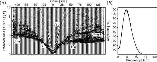
Representative shot gather (a) of the synthetic, viscoelastic, vertical component data from the CCSS model for a shot located at x= 109.98 km, z= 0.045 km, and (b) associated amplitude spectrum. All time domain data have a reduction velocity of 7 km s⁻¹ applied. For display purposes, only the initial 10 s of data and every 25th trace is shown. Labelled arrivals: Pn, first arrivals refracted from the upper mantle; Pg, first arrivals refracted from the upper crust; PmP, wide-angle reflections from the Moho; I, direct arrivals; Rg, Rayleigh waves.

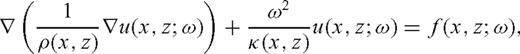
In our study, a pragmatic approach was taken in determining which of the available components of data were used for the acoustic waveform tomography test: Forward modelling with the acoustic wave equation, as in eq. (4), generates a scalar (pressure) wavefield, restricting the modelled waveforms to contain only P waves. However, the viscoelastic modelling scheme used to synthesize the CCSS data generates a vector wavefield, separating the pressure response into vertical- and horizontal-components. Since the vertical-component response of a seismometer is dominated by incident P waves, only the vertical-component data were used. As Operto (2004) point out, a conversion from pressure to vertical particle displacement is strictly required. However, this would also require that the calculation of the Jacobian matrix of the partial derivatives of the vertical particle displacements with respect to the model parameters be implemented within the waveform tomography code, a non-trivial task. The results described below and in Paper II justify this less rigorous approach to waveform modelling, and provide valuable evidence of the efficacy of computationally efficient, approximate (acoustic) methods when undertaking waveform inversion of elastic data.

First arrival traveltime tomography

In all applications of waveform tomography, it is critical to generate a sufficiently accurate starting model in order to allow the misfit function to converge to the global minimum. Previous synthetic experiments in waveform tomography have used data generated in models which were known to the tomographers a priori, such as the Marmousi model (Forgues 1998; Sirgue & Pratt 2004). In many cases the starting model used for waveform inversion was unrealistically close to the true model; for example, both Forgues (1998) and Shipp & Singh (2002) generated starting models for synthetic experiments by extracting the large-scale features from the true model. In other cases, such as the application to the physical scale model described by Pratt (1999), a starting model was derived by using the curved-ray traveltime tomography method described by Pratt (1993).

The principal method used in the analysis of wide-angle seismic data for lithospheric imaging is traveltime tomography. The method has been widely developed, including both 2-D (e.g. Zelt & Smith 1992; McCaughey & Singh 1997; Korenaga 2000) and 3-D applications (e.g. Hole 1992; Toomey 1994; Hobro 2003). Combinations of both refraction (Pg, Pn) and wide-angle reflection (PmP) traveltimes can be used to jointly estimate velocities and interface depths; normal-incidence data can also be combined, and will significantly improve the resolution of the tomographic solution (McCaughey & Singh 1997). Recent work by Sirgue & Pratt (2004) has shown that a starting model derived by the ray-based, first arrival traveltime tomography method of Zelt & Barton (1998) provides a good starting point for waveform tomography. In Zelt & Barton's (1998) method, ray paths are calculated at each iteration of regularized inversion using the finite-difference solution of the eikonal equation (Vidale 1990), modified to handle large velocity contrasts (Hole & Zelt 1995). The regularization generally consists of combined smoothness and flatness constraints. Only the traveltimes of wide-angle refractions (Pg, Pn) are inverted; later arrivals are ignored, including reflections from geologic interfaces (i.e. PmP). Limited to only the first arrivals, boundaries are represented by velocity gradients, and the resulting velocity model is limited to a low-wavenumber solution; the interface structure represents a portion of the high-wavenumber solution. Sirgue (2003) has found the low wavenumbers to be directly related to the linearity of the problem: by beginning waveform tomography with a low-wavenumber starting model, the non-linearity of the inverse problem may be avoided, and the misfit function will be more likely to converge to the global minimum.

For the CCSS data, the Zelt & Barton (1998) method of first arrival traveltime tomography was used to generate the starting model for waveform tomography (Zelt 2004). The first-arrival picks, the 1-D starting model, and the 2-D velocity model from traveltime tomography described here were provided to the authors prior to implementation of waveform tomography. First-arrival times were picked from the vertical-component CCSS data for every receiver of each CSG, for a total of 141 729 picks. Due to the noise-free nature of the data, a picking error was assigned to each pick approximately 1.5 times the sampling rate of 16 ms (i.e. 25 ms). A 1-D starting model for first arrival traveltime tomography was derived based upon an analysis of the time-offset relationship for the entire data set, using the method described in Zelt & Smith (1992), with a nodal spacing of 1 km. The 1-D model is shown in Fig. 3. Below 35 km, a small negative gradient was added to prevent rays from emerging from the bottom of the model. Traveltime tomography was performed with regularization parameters constraining the solution to be smoother in the vertical direction than in the horizontal by a ratio of 4 to 1 (i.e. s_z= 0.25). A goodness of fit parameter, χ², was calculated for each model run, optimally obtaining a final value of χ² approximately equal to 1.0. An average rms misfit of approximately 25 ms was obtained for each of these runs. An average of 8 smoothness-constrained models was taken to determine the final traveltime tomography result, depicted in Fig. 1(b). This result, provided to the authors prior to the CCSS workshop, was used as the starting model for waveform tomography (Brenders & Pratt 2003). The accuracy of the traveltime tomography greatly contributed to the ability of waveform inversion to avoid convergence to a local minimum.

Figure 3

Open in new tabDownload slide

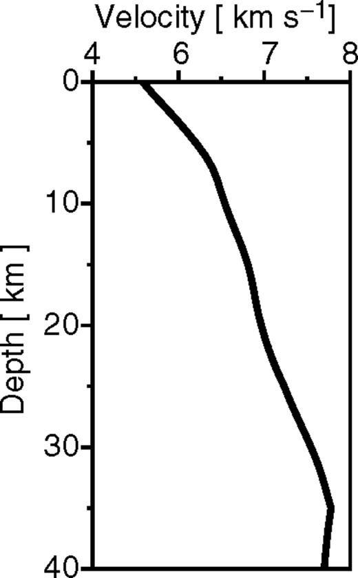
The 1-D starting model obtained by analysis of the first arrival time-offset relationship of the entire CCSS data set. This velocity model was used as the starting model for the first arrival traveltime tomography result in Fig. 1(b).

The 2-D traveltime model in Fig. 1(b) contains features which compare favourably with the large-scale structure of the CCSS model. The low-velocity upper sediment layer has a thickness of approximately 5 km between 50 and 125 km along the model, shallowing towards the right. The anticlinal structure of the upper crust between 175 and 250 km along the model has been partially imaged, and the crust–mantle transition zone has been approximately located between depths of 25 and 30 km throughout the model. The traveltime tomography result does not capture details such as the medium-wavelength velocity perturbations, the lenticular low-velocity zone, or the well-defined crust–mantle transition zone. However, the model obtained from first-arrival traveltime tomography was essential as a starting model for the 2-D, acoustic, frequency-domain waveform tomography method.

Initial forward modelling

Before attempting any waveform tomography, forward modelling is an important step in qualitatively evaluating the starting model and in evaluating whether waveform tomography is likely to succeed. If the observed waveforms are not matched to within a half-cycle by the synthetic data forward-modelled within the starting model, a local minimum in the objective function may be encountered: the steepest descent method used to calculate the model update will attempt to fit the calculated data to the wrong cycle of the observed data, and the tomographic solution may begin to diverge. The results of this forward modelling are also used to scale the acoustic amplitude versus offset response of the real, viscoelastic data, further described below. The 2-D starting model shown in Fig. 1(b) was used for initial, frequency-domain, finite-difference modelling with the acoustic method of Pratt & Worthington (1990) and Jo (1996). For the group and phase velocities of waves propagating within a given model to be at least 95 per cent accurate, a grid spacing (Δ) is chosen to have a minimum of four gridpoints per smallest wavelength,

10

where λ_min=c_min/f_max is the minimum wavelength present in the model for a given minimum velocity, c_min, and maximum frequency, f_max (Jo 1996). Estimating the minimum expected velocity in the model to be 4 km s⁻¹, for a maximum modelling frequency (f_max) of 1.0 Hz, a cell size of 1.0 km or smaller is necessary. For accurate modelling of wave propagation up to a maximum frequency of 6.25 Hz, a model 250 km long by 40 km deep must be discretized on a grid with spacing Δ= 0.16 km. Arbitrary positioning of multiple sources or receivers within individual cells is implemented by the using the method described by (Hicks 2002). Table 2 lists the different finite-difference grids used in this paper.

Table 2

Open in new tabDownload slide

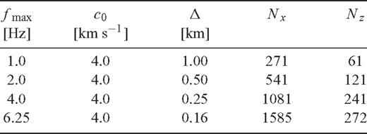
The sizes of the finite-difference grids defining the velocity model for forward modelling and waveform tomography, calculated using eq. (10), for four maximum frequencies. The total number of gridpoints includes ‘absorbing’ boundaries.

Following examination of the amplitude spectra of each of the individual shot gathers, as in Fig. 2(b), we initially chose f_max= 2.0 Hz, and interpolated the velocity model from first-arrival traveltime tomography (Fig. 1b) onto the finite-difference grid defined in Table 2. We used a two-excursion Keuper wavelet as a source function, with a dominant frequency of 0.556 Hz (and a peak frequency close to 2 Hz), thus forcing the bandwidth of the source to match the maximum frequency allowable on the finite-difference grid. This source signature was very approximate, intended only to demonstrate that our starting model could match the waveforms of the CCSS data to within a half-cycle.

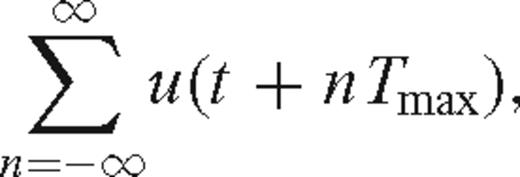
To compare the CCSS data to the data calculated by modelling with frequency-domain methods, frequency-domain modelled data must first be transformed into the time domain using a discrete inverse Fourier transform. Because of the periodicity of the discrete transform, frequency-domain modelling methods will induce ‘time wraparound’ (or ‘time aliasing’) in the time-domain data if the frequency sampling interval is not sufficiently small. A frequency sampling interval was chosen according to Δf= 1/T_max, where T_max is the length of the seismic trace. For a time function f(t), discrete frequency-domain data will be transformed into an aliased time function of the form f(t+nT_max), where n is an integer from −∞ to ∞. Aliasing can be suppressed by using a value of T_max large enough for any late signals to have decayed.

Since choosing a large value of T_max is computationally expensive, as this implies a small value of Δf, to suppress time aliasing we use a method developed by Mallick & Frazer (1987) for the reflectivity method. In eq. (4), each element in the vector u(ω) is the Fourier transform of a time-domain seismogram, u(t). To obtain u(t), for each receiver location we compute a discrete series of u(ω) with a range of frequencies using eq. (4). By using a discrete inverse Fourier summation, we obtain the periodic time-domain signal,

11

where T_max= 1/Δf, and Δf is the frequency interval in the computed values of u(ω). Thus, if the seismogram u(t) is non-zero for t > T_max the result will be corrupted. To prevent this, we can instead compute u(ω′) =u(ω+i/τ), instead of u(ω), by simply modifying eq. (4) to substitute

12

a complex-valued angular frequency, for ω in all modelling equations. Because u(ω′) is just the Fourier transform of u(t)e^−t/τ (the damped time-series), after discrete inverse Fourier summation we obtain

13

Thus, by using a complex-valued angular frequency, the time-domain seismogram has been multiplied by a decaying exponential function, with each successive time-aliased component of the original seismogram multiplied by a smaller value. To recover an approximation of the original seismogram we multiply the result by the factor e^t/τ, producing

14

For the unaliased component (n= 0), the original time-series is recovered. For all positive values of n, the signal is attenuated by an increasing factor—attenuated by a minimum of e. The method fails if the seismogram has non-zero values for negative times (n < 0), as the negative time samples will be amplified. In our forward modelling, we chose an initial decay factor of τ≈ 0.4 ×T_max= 16 s, where T_max= 40 s is the total trace length of the reduced time CCSS data.

Forward modelling was performed for 51 shot gathers, with 278 receivers per shot gather, equivalent to a shot spacing (Δs) of 5.0 km and a receiver spacing (Δr) of 0.9 km. For comparison to the original CCSS data, time-domain traces were generated with a total trace length (T_max) equal to 40 s reduced time, using a reduction velocity of 7 km s⁻¹. Modelling in the frequency-domain was performed with a frequency sampling interval, Δf, calculated to be 1/T_max= 0.025 Hz. Table 3 lists the other parameters used to forward model within the starting velocity model. The frequency-domain data were transformed by inverse FFT to the time domain; after padding of the 80 discrete frequencies a pseudo-sampling rate of approximately 19 ms was achieved, and subsequently resampled to the 16 ms sampling rate of the CCSS data. In Fig. 4, the CCSS data waveforms (low-pass filtered to 2.0 Hz) are compared with our initial 2 Hz synthetic data for a sample shot gather. Upon first inspection, the match between waveforms seems poor. However, at this stage we were only concerned with being able to model the first arrival to within a half-cycle, and not the entire waveform. For the CSG in Fig. 4(d), several important features can be observed:

Table 3

Open in new tabDownload slide

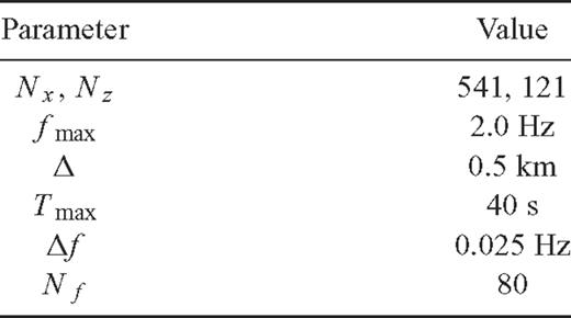
Parameters for frequency-domain forward modelling in the starting velocity model.

Figure 4

Open in new tabDownload slide

Comparison of the viscoelastic CCSS data and the acoustic, synthetic, forward modelled data for the shot gather located at x= 109.98 km, z= 0.045 km along the model: (a) CCSS data sub-sampled by using only every 10th receiver (Δr= 0.9 km) (b) low-pass filtered to 2.0 Hz, (c) time windowed to 3 s after the first arrival and offset weighted to zero traces with less than 25 km offset, (d) synthetic data from forward modelling in the starting model with a Keuper wavelet with a maximum frequency of 2 Hz. Note that no attempt has been made at this stage to match the source signature of the CCSS data.

• (i)

  First arrivals are matched to within a half-cycle.

• (ii)

  Weaker amplitudes in the secondary arrivals between 80 and 110 km offset corresponded to weaker amplitudes in Fig. 4(c) centred at 100 km offset.

• (iii)

  The relative change in slope of the first arrivals has been matched, notably between 30 and 50 km offset and −90 and −75 km offset.

Similar comparisons were made for each of the 51 shot gathers. These initial forward-modelling results were encouraging enough to continue to implement waveform tomography with these data.

Data preconditioning

When working with real seismic data, trace sampling of the input data is sometimes required to eliminate data of poor quality when using waveform tomography (e.g. Operto 2004; Ravaut 2004). We sub-sampled the CCSS data set within the CSGs in order to reduce the necessary computational resources. This was achieved by increasing Δr from 0.09 to 0.9 km for the CCSS data, thus reducing the amount of data being computed in the initial applications of forward modelling and waveform inversion. The CCSS data were low-pass filtered to 2 Hz initially to allow direct, qualitative comparison between forward-modelled waveforms and the CCSS data, since the finite-difference grid restricted modelling frequencies to this maximum value. Fig. 4(a) shows a CSG of the CCSS data, sub-sampled at Δr= 0.9 km (every 10th receiver). Fig. 4(b) shows this same shot gather following application of a low-pass Ormsby filter, with corner frequencies of 0–0–1.8–2.0 Hz.

To add stability to the inversion and to remove phases in the data which cannot be modelled by the acoustic finite-difference method, such as shear-wave arrivals and mode conversions, the input CCSS data were windowed in time to include only waveforms occurring within a 3 s window (T_win) after the first arrival. This window was tapered by 32 samples at each end to improve the frequency-domain characteristics of the waveforms. The tapered window was applied to the sub-sampled, low-pass filtered data set, as shown in Fig. 4(c).

Since the near offset waveforms were dominated by Rayleigh modes, it was important to preclude these data from the acoustic inversion algorithm. An offset-dependent cosine taper varying between 0 and 1 was used to suppress data residuals from the near offsets. By inspection of the time-windowed data, we observed that data from offsets of less than 18 to 25 km, within 3 s of the first arrival, have waveforms contaminated by elastic modes. The taper was set to zero data below 18 km, increasing to a value of one at 25 km. This taper was applied to the sub-sampled, low-pass filtered, time-windowed data of the CSG shown in Fig. 4(c). This figure depicts the final pre-conditioned data used for input into the waveform inversion process.

Inspection of the original vertical-component time-domain data and our acoustic-modelled time-domain data showed a significant disparity in the variation of the amplitudes of the seismic traces with offset. Although both data sets exhibited a general decay in amplitude with increasing offset, the relative amplitude differences between respective near-offset and far-offset traces is extreme. This difference is largely due to the difference in radiation patterns for the elastic-wave vertical point-force source used to generate the CCSS data, as compared with the acoustic-wave (explosive) source used in our forward modelling scheme. Disparity in the inelastic attenuation factors associated with the true model, compared to the constant values used in our acoustic wave-equation method, also plays a role, as does the receiver antenna pattern. To invert data from all offset ranges, we found it essential to scale the amplitudes of the CCSS data to match the amplitude-versus-offset decay of the forward-modelled synthetic data (in addition to suppressing the near offsets dominated by Rayleigh waves and high amplitudes).

The sub-sampled, time-windowed CCSS data and the forward-modelled data were sorted into 51 equal offset bins, and the rms amplitudes of the seismic traces were calculated for each bin. We parametrized the decay of the rms amplitudes with offset using a simple exponential-decay function. The parameters were obtained from a linear regression of the log rms amplitudes as a function of offset, x, yielding two straight-line equations, ax+b for the synthetic log rms amplitudes, and a′x+b′ for the CCSS log rms amplitudes. Thus, the decay of the synthetic and CCSS rms amplitudes is given by e^a′x+b′ and e^ax+b, respectively. We wanted to find a simple formula for correction factors as a function of offset, say f(x). Working only with the exponential-decay functions,

15

i.e. another simple exponential-decay function. This simple, two-parameter expression has the advantage of being non-negative, an important consideration when working with rms amplitudes.

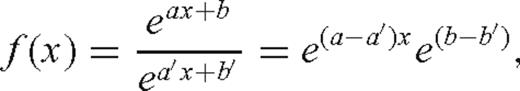
Fig. 5(a) shows the variation of the log rms amplitudes for the CCSS data, low-pass filtered to 2 Hz. Fig. 5(b) shows the variation of the log rms amplitudes for the synthetic acoustic data, forward modelled to 2 Hz within the starting velocity model. The relative disparity between the two data sets is evident upon examination of the vertical scale of each plot. Multiplying the CCSS amplitudes by the scaling factor calculated in eq. (15) allowed both the CCSS data amplitudes and the forward-modelled data amplitudes to be plotted on the same vertical scale, displayed in Fig. 5(c). The calculated scaling function was applied to the sub-sampled, low-pass filtered, time-windowed CCSS data. Finally, the amplitude corrected CCSS data were transformed by Fourier summation (using the complex-valued frequency described by eq. (12), with the value of τ= 0.16 chosen above), and the individual frequency components were extracted for subsequent inversion with waveform tomography.

Figure 5

Open in new tabDownload slide

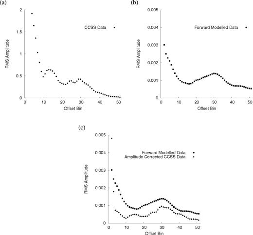
Amplitude variation with offset for (a) the CCSS data, (b) the synthetic data forward modelled in the starting velocity model, and (c) the amplitude scaled CCSS data and the forward modelled data. The rms amplitudes for the CCSS data were originally much larger than those of the synthetic, forward modelled data. Note the effect of the near offset amplitudes.

Waveform tomography strategy

The non-linear nature of the waveform inverse problem implies that local minima may be encountered. A strategy to mitigate this non-linearity is required. Two such strategies for waveform tomography have been a layer-stripping approach, such as that advocated by Pratt (1996), or a multiscale approach proceeding from low wavenumbers to high, using low temporal frequencies first, and refining with higher frequency data (Bunks 1995). The latter approach is more appropriate for a wide-angle survey, as the long-offset data are more sensitive to the low wavenumbers in the model (Sirgue 2003). Although the layer-stripping approach has proven feasible when using waveform tomography for sub-basalt imaging (Sirgue & Pratt 2002), a multiscale approach is more powerful when low frequencies are available. To optimize the convergence of waveform tomography, we adopted the multiscale approach. Several successful examples of time-domain waveform inversion (Shipp & Singh 2002) and frequency-domain waveform tomography (Sirgue & Pratt 2004; Ravaut 2004; Operto 2004) have also followed this strategy.

The multiscale approach also offers a computational advantage: by initially inverting low frequencies and sequentially increasing the inversion frequency, the finite-difference grid spacing used to represent the velocity model is adaptable to specific frequencies. Coarser grids can be used for the lower frequencies, and finer grids for higher frequencies. Using coarse grids at the early stages of waveform tomography allows for relatively inexpensive computation and rapid confirmation that the solution is converging towards the critical global minimum. In addition, since low frequencies tend to have a more linear relationship with the low wavenumber components of the model, recovery of these components at the early stages of waveform tomography assists in mitigating the non-linearity of the problem (Sirgue 2003). The strategy for full waveform tomography is summarized in Table 4, and subsequent references to the strategy will be made according to the stages listed in this table.

Table 4

Open in new tabDownload slide

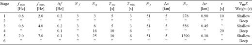
The strategy for full waveform tomography: N_g groups of N_f frequencies are simultaneously inverted for a maximum of 5 iterations, before moving onto the next group. The total number of iterations for each stage is equal to 5 ×N_g. Preconditioning of the gradient image with depth was performed according to the above schedule, and low-pass wavenumber filtering of the gradient was performed for all stages.

Waveform tomography of the CCSS data set began with an examination of representative amplitude spectra of the shot gathers, such as that depicted in Fig. 2, and choosing the lowest frequency of data available with significant energy (0.8 Hz). The velocity model from first-arrival traveltime tomography (Fig. 1b) provided the minimum velocity expected in the final model, approximately 4 km s⁻¹. Choosing several low frequencies, eq. (10) was used to calculate the size of the cells of the finite-difference grids necessary for the inversion of frequencies up to a maximum value. For a model 250 km wide and 40 km deep, these values of Δ allowed the number of gridpoints to be calculated, as summarized in Table 2.

The CCSS data were originally modelled with a free surface, as evidenced by the Rayleigh modes present in Fig. 2. To effectively prevent reflections and diffractions at the corners of the model, where the 45 degree one-way propagators are less effective (Clayton & Engquist 1977), we assigned gridpoints a finite Q value at the corners of the model, and kept attenuation equal to zero in the interior region of the model. In the first four stages outlined in Table 4, the total finite-difference grid size included a 10 km boundary on each side. For the highest frequencies inverted, using the finest sampled finite-difference grid, this boundary was reduced to a minimum of 10 gridpoints on all sides.

Prior to stage 1 of waveform tomography, an initial source estimate was calculated from the band-limited data using the starting model from first-arrival traveltime tomography and the method described by eq. (8). Data frequencies from 0.8 Hz to 4 Hz were used. The length of the source signature, T_src, was chosen such that T_src≥T_win, covering the time window of CCSS data used in waveform tomography. The ‘design window’ used in estimating the source wavelet is longer than the expected length of the source wavelet from the time-windowed data; this is consistent with the practice of predictive deconvolution. In addition, this had the effect of reducing time aliasing in the recovered source waveform estimates. T_src was initially chosen to be 5 s, 40 per cent longer than the time window of 3 s applied to the CCSS data. An identical source signature was used for each of the 51 sources. After each subsequent stage of the ‘full’ waveform tomography strategy, the source signature was re-estimated using the updated velocity model. As the strategy progressed to a wider range of frequencies, a more realistic looking source was obtained, as shown in Fig. 6 for three subsequent stages of the waveform tomography strategy. The true source wavelet was not made available to us, and would differ from the inverted source signature due to free-surface ghosting and near-surface scattering.

Figure 6

Open in new tabDownload slide

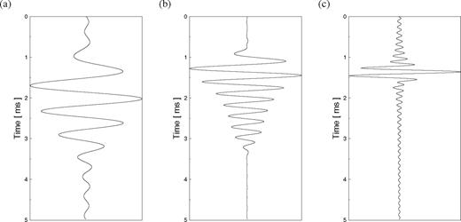
Source signatures extracted from the data by waveform inversion, (a) using the traveltime tomography result as a velocity model, containing frequencies from 0.2 to 2.0 Hz, (b) using the velocity model from Stage 2 as a velocity model, containing frequencies from 0.2 to 4.0 Hz, and (c) using the velocity model from Stage 4 as a velocity model, for frequencies from 0.1 to 7.0 Hz.

In addition to reducing the effects of time aliasing, a complex-valued ω, as in eq. (12), also allows damping of the waveform residuals after the first arrival. An iteration of waveform inversion is more likely to converge if we can force the early arrivals in the synthetic waveforms to match the first arrivals present in the CCSS data. The risk of cycle skipping is high in a non-linear problem, and the early arrivals represent the most linear component of the wavefield, as well as containing those wavefield components most likely to be correctly predicted within a starting model obtained using first-arrival traveltime tomography (Sirgue 2003). Increasing the weighting of the early arrivals in the data residuals was accomplished by damping the amplitudes of the later arrivals in the residual data. In the frequency-domain, multiplication of the residual wavefields by a factor of e^−t/τ allows us to damp the late arriving energy (e.g. eq. 14). However, for seismic traces recorded at non-zero offsets, the first-arrival time of the recorded signal will be non-zero, and the starting point of the damping function must be shifted. By pre-multiplying the residuals with a factor of e, the weighting factor can be set equal to one at any desired arrival time t₀. For each frequency component of the data, this factor was applied using values of t₀ approximated for each seismic trace by dividing the offset of the trace by the minimum velocity present in the model. After some initial tests with τ= 16 s, a decision was made to relax the time damping in order to improve the qualitative match of the observed and synthetic waveforms. The factor of τ was set equal to 10 s for stages 1 to 3 of the waveform tomography strategy (see Table 4), and subsequently increased to 20 s (when the length of the time window applied to the CCSS data was increased to 6 s).

Stage 1 of waveform tomography was performed using waveforms from 278 receivers per CSG, with Δr= 0.9 km and Δs= 5.0 km. Temporal frequency components from 0.8 to 2 Hz were used, sequentially inverted in overlapping groups of three frequencies, as listed in Table 5. For full waveform tomography, sampling theory dictates that the interval between frequencies, Δf, should satisfy the requirement that Δf≤ 1/T_win, where T_win is the length of the data time window being used. Since T_src≥T_win, this requirement is satisfied by choosing Δf= 1/T_src. In addition, this is consistent with the frequency sampling interval used to calculate the source signature. Stage 2 of waveform tomography used the same frequencies, but in this case we preconditioned the intermediate gradient image by increased weighting with increasing depth. Depth weighting of the gradient effectively forced the velocity model update to be more emphasized within the deeper portions of the model than in the shallower portions. We also suppressed the gradient within 1 km of the source, necessary due to the singular nature of the Green's functions at their origins. The weighting function consisted of a cosine taper defined by four corner points equivalent to the depths where the weighting factor tapered from 0 to 1, and 1 to 0, respectively. Two weighting functions were used, corresponding to either shallow or deep weighting of the gradient. For each stage, the depth weighting function used is indicated in Table 4. With shallow gradient-weighting, the gradient was weighted from a value of 0 at 0 km depth, tapering to 1 at 1 km depth, and remaining at this value throughout the entire depth of the model. For deep-gradient weighting, the weighting factor tapered from 0 at 0 km depth to 1 at a depth of 60 km, below the bottom of the model.

Table 5

Open in new tabDownload slide

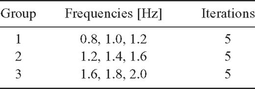
Schedule of frequencies used in Stages 1 and 2 of the ‘full’ waveform inversion of the CCSS data. For each frequency group, the highest frequency of the previous group was used as the lowest frequency of the next group. Similar schedules were followed in Stages 3 and 4 (0.8 to 4.0 Hz, Δf= 0.2 Hz), and in Stages 5 and 6 (2.0 to 7.0 Hz, Δf= 0.1 Hz).

Stages 3 and 4 required the interpolation of the updated velocity model from stage 2, sampled at Δ= 0.5 km, onto a finer grid of Δ= 0.25 km. A new source signature was estimated for frequencies of 0.8 to 4.0 Hz, and waveform tomography continued, using 8 groups of three frequencies from 0.8 to 4 Hz, again with Δf= 0.2 Hz. In stages 3 and 4 the number of receivers was increased to 556 per CSG (with Δr decreasing to 0.45 km). Stage 4 was a second pass of frequencies from 0.8 to 4.0 Hz, again weighting the gradient with depth. In an attempt to fit the later arrivals in the waveforms, the time window was increased to 6 s, and the length of the source signature was increased to 10 s. This dictated a decrease in Δf to 0.1 Hz. The starting point of the offset-dependent taper was also increased from 18 to 20 km, to avoid fitting Rayleigh mode events now appearing in the larger window.

Finally, the velocity model was interpolated onto a grid with Δ= 0.16 km, and a source signature with T_src= 10 s was calculated. In stage 5, frequencies from 2.0 to 7.0 Hz were inverted in simultaneous blocks of three, again with Δf= 0.1 Hz. Although the data contain significant energy up to frequencies of 10–12 Hz (as shown in Fig. 2b), as described earlier, the computational limitations of the finite-difference grid used for waveform modelling precluded accurate modelling above 7.0 Hz. Inversion of larger frequencies could have been accomplished if sufficient computational resources, allowing factorization of the larger finite-difference grids, had been available. Data from 1390 receivers, with Δr= 0.18 km were used, with a 6 second time window around the first arrival and an offset weighting of 0 at 20 km, increasing to a value of 1 at 27 km. Stage 6 was performed with depth weighting applied to the gradient for frequencies from 2.0 to 7.0 Hz.

As part of our multiscale approach, low-pass filtering of the gradient image was performed by eliminating wavenumbers greater than k_{x max} and k_{z max}, defining the boundaries of an ellipse in the wavenumber domain (Sirgue 2003). The intended effect of this filter was to suppress the unstable, high-wavenumber components in the model, and to weight the low-wavenumber components to enhance convergence and effect larger scale model updates. During the inversion of each group of three frequencies, the wavenumbers of the gradient image were preconditioned using a spatial low-pass filter in the wavenumber domain. Values of k_{x max} and k_{z max} were chosen based upon calculation of the maximum possible wavenumber for the maximum frequency in the current stage of the inversion. As Wu & Toksöz (1987) demonstrated, for data of a given frequency, f, in a model with a minimum velocity, c_min, the maximum theoretical wavenumber spectrum coverage is bounded by 2f/c_min (we distinguish wavenumber, k (in km⁻¹), from angular wavenumber (rad km⁻¹), which would include a factor of 2π). For each group of three frequencies, in order to suppress lateral variations preferentially over vertical variations within the image, the values of k_{x max} were adjusted to be approximately five times smaller than those of k_{z max}. A taper zone in k_x, k_z space was applied to prevent artefacts from being introduced by the filter. As the tomography progressed to higher frequencies, the wavenumber filter was relaxed, allowing larger wavenumbers to contribute more in order to improve the spatial resolution of the velocity model. Fig. 7(a) shows the gradient of the misfit function for the inversion of 0.8, 1.0, and 1.2 Hz data with neither depth weighting, nor wavenumber bandpass filtering, yet applied. In Fig. 7(b), both the depth weighting and wavenumber bandpass filtering preconditioning operators have been applied to the gradient, and the gradient image now updates large areas of the model due to the predominance of low wavenumbers.

Figure 7

Open in new tabDownload slide

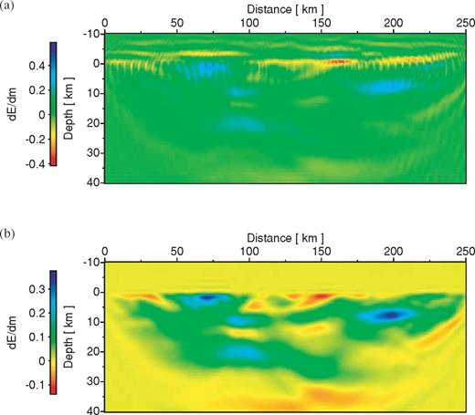
Images of the gradient of the misfit function for the first iteration of frequencies 0.8, 1.0, and 1.2 Hz, (a) before preconditioning and (b) after preconditioning has been applied. Preconditioning of the image includes both weighting with depth and low-pass filtering in the wavenumber domain. The model begins at −10 km due to the absorbing boundary conditions used.

The inversion of each frequency group was stopped after 5 iterations per group; beyond this we observed a lack of significant reduction of the misfit function, and further iterations would have led to excessive computational costs (especially at the higher frequencies). It is difficult to assign stopping criteria in waveform inversion, due to the unknown level of data errors. Data errors in the seismic waveforms are primarily governed by ‘modelization errors’ (see Tarantola 1987), caused by errors in the forward modelling algorithm. We use acoustic modelling to describe pressure-field waveforms, but the ‘true’ CCSS data were viscoelastic, vertical particle-velocity wavefields. Modelization errors cannot be easily estimated, and therefore a chi-squared (or similar goodness-of-fit) stopping criteria cannot be used. Additional quality control of the inversion results are given by repeated forward modellings within the updated velocity models.

Forward modelling after stages 2 and 4 allowed a comparison of the original time-domain data with frequency-domain forward modelling through the updated velocity models. These velocity models predicted the CCSS data waveforms well for each chosen frequency. These modelling stages also allowed the values of the amplitude scaling factor (see eq. 15) to be recalculated for an updated model and an increased number of receivers. Forward modelling in the final velocity model, Fig. 1(c), after stage 6 of waveform tomography, was performed with 51 shots and 1390 receivers (Δr= 0.18 km), for frequencies up to 7.0 Hz, using a source signature calculated from the CCSS data by the method described in eq. (8). These synthetic data are shown in Fig. 8(a) for the shot gather corresponding to Figs 4(a) to (d). The corresponding CSG of the CCSS data is presented in Fig. 8(b), sub-sampled and low-pass filtered to 7.0 Hz. As expected, very good agreement was observed in the waveforms near the first arrival at all offsets. Good agreement between the synthetic data and the CCSS data was also observed in the later parts of the waveforms (green arrows). Some data phases observed in the CCSS data, including purely elastic phases such as Rg and converted wave arrivals, were absent from the synthetic data (red arrows).

Figure 8

Open in new tabDownload slide

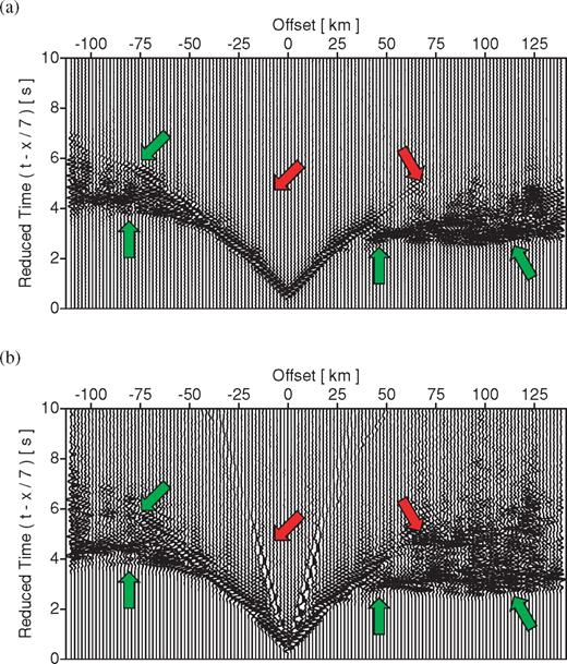
Comparison of the acoustic, synthetic, forward-modelled data and the viscoelastic CCSS data for the shot gather located at x= 109.98 km, z= 0.045 km along the model: (a) forward modelled to 7.0 Hz in the final velocity model from waveform tomography, using 51 shots and 1390 receivers (Δr= 0.18 km) and a source inverted from the CCSS data, (b) CCSS data low-pass filtered to 7.0 Hz. Green arrows indicate good agreement between the forward-modelled data and the CCSS data in the first arrivals located at near and far offsets, and in the later arrivals at far offsets; red arrows indicate poor agreement, including Rg phase not modelled by the acoustic data, and some later arrivals, initially interpreted as PmP reflections. Both CSGs have been trace normalized for display purposes.

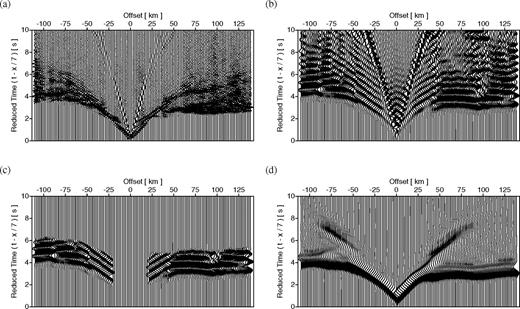
In the absence of borehole logs or some other constraint on the velocity model, in a real seismic survey the comparison of synthetic and observed waveforms is the only objective form of quality control available. Fig. 9 presents detailed time-domain overlays of the waveforms from the low-pass filtered, amplitude-scaled, viscoelastic CCSS data and the acoustic, synthetic data, forward modelled to 7.0 Hz, for the shot gather previously described. Using the source signature estimated from the velocity model in Fig. 1(c), forward modelling was performed in both the starting model (Fig. 1b) and in the final waveform tomography result. Results from forward modelling in the starting model are presented in Fig. 9(a) for negative offsets between −109 and −25 km, and in Fig. 9(b) for positive offsets between 25 and 140 km, for waveforms recorded from 2 to 6 s reduced time. Results from forward modelling within the final model are presented in Figs 9(c) and (d), for identical offsets and trace lengths. For display purposes, traces are spaced every 1.8 km, and first arrival times are displayed for reference purposes. These time-domain overlays clearly illustrate the improvement in data-fitting obtained in the inversion: Figs 9(a) and (b) demonstrate the ability of the starting model to accurately model the first arrival traveltimes, but not the detailed amplitude and phase behaviour of the waveforms. The improvement when using velocity models calculated from waveform inversion is illustrated by Figs 9(c) and (d), demonstrating the ability of an acoustic forward-modelling scheme to model the complexities present in viscoelastic waveforms of the early arrivals, and well into the coda, including the amplitude behaviour. For example, the decreased amplitude of the positive offset traces in Figs 9(b) and (d) is likely caused by the creation of a shadow zone due to the low-velocity zone present in the CCSS model.

Figure 9

Open in new tabDownload slide

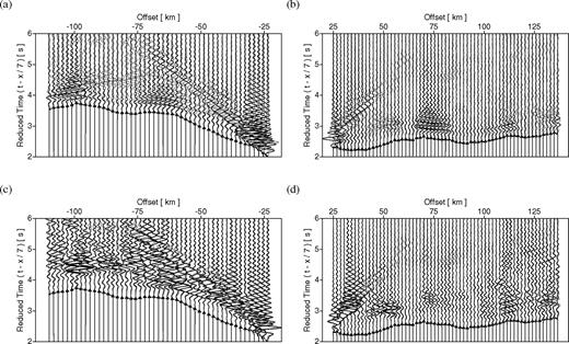
Shot gather of the viscoelastic CCSS data (grey), located at x= 109.98 km along the model, for signed offsets of −109 to −25 km and 25 to 140 km, low-pass filtered to 7 Hz, overlain on (a), (b) the acoustic, synthetic data (black), forward modelled to 7 Hz in the starting model, and (c), (d) synthetic data forward modelled to 7 Hz in the final model from waveform tomography, Fig. 1(c), using a source signature inverted from the real data and final model. First arrival times are plotted as triangles joined with a dashed line. Data are plotted with the same scaling, and without trace normalization.

Traveltime tomography does not explain all of the information present in the CCSS data. The parts of the data not sufficiently explained by the models are illustrated by the time-domain residuals in Fig. 10. Figs 10(a) and (b) show residuals from the starting model, and Figs 10(c) and (d) show residuals calculated using the result from stage 2 of waveform tomography. All residuals are plotted with the same scaling, without trace normalization. A significant decrease in the residuals is observed between 50 and 75 km offset, within 0.5 s of the first arrival, though the near-offset traces are still dominated by R_g phases. Figs 10(e) and (f) show the results from forward modelling in the result from stage 4 of waveform tomography, and Figs 10(g) and (h) depict the final residuals. As the waveform tomography strategy progressed, waveforms were better matched to increasingly later times, indicated by the near-zero values of the residuals immediately following the first arrivals. Significant energy remains throughout each stage of waveform tomography at approximately 4.5 s between 70 and 90 km offset, and elsewhere due to the presence of R_g phases (i.e. where identified by red arrows in Fig. 8). Non-zero residuals represent aspects of the CCSS data which cannot be explained by either traveltime tomography or waveform tomography with the acoustic wave-equation. Waveform inversion with the viscoelastic wave equation may succeed in reducing these residuals if they represent converted waves or other elastic phases.

Figure 10

Open in new tabDownload slide

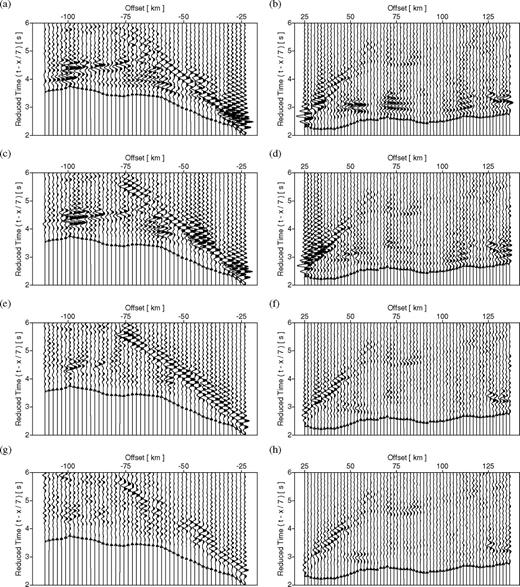
Residuals calculated for the shot gather located at 109.98 km along the model, for offsets of −109 to −25 km and 25 to 140 km, respectively, for synthetic data forward modelled to 7 Hz in (a), (b) the starting model, (c), (d) the result from stage 2 of waveform tomography, (e), (f) the result from stage 4 of waveform tomography, and (g), (h) the final waveform tomography result. First arrival times are plotted as triangles joined with a dashed line. The source signature used was inverted from the real data and final model. Residuals are plotted with the same scaling, and without trace normalization.

Final results

The final velocity model calculated using the multiscale strategy of full waveform tomography is presented in Fig. 1(c). This model matches both the large- and intermediate-scale features of the true model to a resolution of the order 1 km (estimated from a posteriori comparison with the true model). The model includes the low-velocity zone between 190 and 215 km along the model, and the detailed structure of the crust–mantle transition. The recovery of the shallow low-velocity zone is important, as this feature was completely absent in the starting model from traveltime tomography, Fig. 1(b). The crust–mantle transition is well imaged within the centre of the model, but is smeared to shallower depths by artefacts along the outer 50 km of both sides of the model. A near-vertical feature located at 90 km along the model is visible, albeit with some gaps. The heterogeneity within the upper crust is generally well imaged, especially within the central 150 km of the model.

Results from the intermediate stages of the full waveform tomography strategy are shown in Fig. 11 as 1-D vertical velocity profiles for surface locations at 79.7 km, 140.5 km, and 199.8 km. Profiles were taken from the starting model (Fig. 1b) and the velocity models after stages 2, 4, and 6 of waveform tomography. A gradual introduction of high-resolution features can be observed as the strategy progresses, indicating waveform tomography is adding structure and complexity to the starting model as higher-frequency components of the data are included in the inversion, and as the wavenumber filtering is relaxed. Nevertheless, the most significant changes to the velocity model were made during the initial inversion of the lowest frequencies (0.8, 1.0, and 1.2 Hz). The profile at 79.7 km shows intermediate-scale, heterogeneous, upper crustal velocity structures between 2 and 16 km, a slightly more homogeneous lower crustal velocity structure between 16 and 25 km, a relatively sharp transition between lower crust and mantle velocities between 25 and 28 km, and a slightly heterogeneous mantle velocity layer below 28 km depth. The starting model (long dashed line) shows only a gradual increase in velocity with depth, and is blind to the low velocity, near-surface structures resolved by full waveform tomography. At a surface location of 140.5 km, the velocity profile indicates an oscillatory transition between sedimentary and upper crustal velocity structures between 3 and 10 km depth, followed by a relatively smooth increase from upper to lower crustal velocities between 10 and 26 km, where a relatively sharp transition to the upper mantle velocity structure is observed. A significant low-velocity zone within the upper crust is resolved between 4 and 8.5 km depth in the profile at 199.8 km, followed by a sharp transition to lower crustal velocities between 12 an 14 km, and a heterogeneous transition to the upper mantle velocities beginning at 26 km depth. Overall, the velocity model result from waveform tomography represents a dramatic improvement in spatial resolution over the result from traveltime tomography. Near-surface, low-velocity structures were very well imaged, as were the crustal velocities within the central portion of the model. The resolution of velocity structure within the mantle is somewhat limited due to a combination of high velocities and a lack of illumination from wide angles.

Figure 11

Open in new tabDownload slide

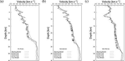
The iterative effect of the ‘full’ waveform tomography strategy used is shown by velocity profiles at (a) 79.7 km, (b) 140.5 km, and (c) 199.8 km along the starting model, the updated velocity models after stages 2, 4, and 6 (as described in Table 4), and the true model. Increased spatial resolution is evident as the waveform tomography strategy progresses.

Computational considerations

All calculations were performed on a PC-based workstation equipped with a 2.8 GHz Pentium IV CPU and 4 Gb of RAM. Computation times per iteration of waveform tomography varied based upon the number of sources and receivers used and the size of the finite-difference grid. Wavefields within the starting model were computed up to 2 Hz for 51 sources and 278 receivers at a rate of 9 s per frequency interval of 0.025 Hz, for a total forward modelling time of 12 min. Inversion of frequencies from 0.8 to 2.0 Hz, for 51 sources and 278 receivers, also on a grid of 541 × 121 nodes, required a computation time of of 44 min, or 160 s per iteration of three frequencies. Inversion of 2.0 to 7.0 Hz, for 51 sources and 1390 receivers, on a grid of 1585 × 272 nodes, took 48.6 min per iteration using three frequencies, for a total computation time of approximately 70 hr. Total computer time for all stages of the waveform tomography strategy was approximately 187.4 hr, but with human interaction and forward modelling (for quality control) factored in, the total time was extended to slightly more than 13 d. For comparison, In Paper II, we describe efficient waveform tomography of the CCSS data set. Using four carefully selected data frequencies, the efficient waveform tomography method recovered a nearly equivalent velocity model in only 21.93 hr, a savings in computational cost of 88.3 per cent.

Discussion and Conclusions

Waveform tomography was applied in a blind test of imaging methods using a 2-D, synthetic, wide-angle seismic data set. The data were generated in a realistic, viscoelastic, crustal geology model 250 km long and 40 km deep. The velocity model calculated via waveform tomography correctly imaged the long- (10 km) and intermediate- (1 km) wavelength features of the crustal model, including a significant near-surface low-velocity zone (invisible to traveltime tomography methods), heterogeneity in the upper and lower crust, and an accurate image of the crust–mantle transition. This model was originally presented at the CCSS workshop in Blacksburg, Virginia, October 2003 (before the true model was revealed). These results provide evidence for the efficacy of applying acoustic, frequency-domain waveform tomography to the early arrivals of viscoelastic, wide-angle data. Furthermore, the experiment described in this paper was performed with third-party seismic data; a priori knowledge of the true source signature and velocity model was minimal. The goal of lithospheric imaging is to obtain an accurate, physical parametrization of the subsurface: elastic data is acquired on the surface with multicomponent seismometers and little a priori knowledge of the subsurface. Waveform tomography with the acoustic wave equation, implemented in the frequency domain, represents a cost-effective candidate solution to this problem: the inverse problem embodied by a real seismic experiment.

Results from the blind test using adaptive traveltime tomography were also presented at the workshop, and are summarized in Trinks (2005). Starting from a linear velocity gradient, they presented a traveltime tomography model calculated using an adaptive model parametrization, which yielded superior results to a model calculated using a non-adaptive parametrization. Trinks (2005) were able to achieve a fairly good resolution of the large-scale features of the CCSS model, but were unable to fully resolve the intermediate-scale velocity structures. Traveltime tomography provides accurate, representative average velocities, but does not enable accurate imaging of medium and small scale heterogeneities.

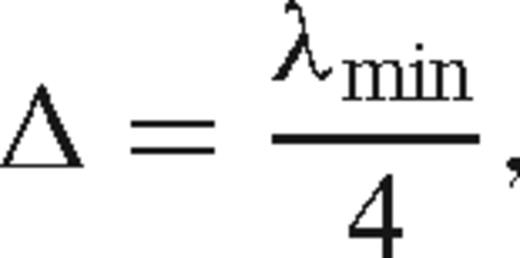
Ray theory, the basis of traveltime tomography, is inherently limited by high-frequency, asymptotic approximations. Additional limitations to both traveltime and waveform methods exist where ray coverage is sparse. The velocity model recovered by full waveform tomography presented in Fig. 1(c) exhibits some smearing of the image at the edges of the model, but nonetheless includes intermediate and some small scale features not visible in the traveltime tomography result. Smearing of the final tomography image is unavoidable due to the finite survey geometry employed. Traveltime methods can produce smooth images, but they are limited to a resolution on the order of , where L is the total path length (Williamson 1991). Although reflection phases may allow the localization of significant geological interfaces, waveform tomography can generally resolve to order λ (Pratt 1990).

The absence of significant noise in the CCSS data set, the correspondingly small first-arrival picking errors (25 ms), and the final traveltime misfit (25 ms) of the velocity model from traveltime tomography may not be representative of a real, crustal-scale seismic data set. To avoid convergence to a local minimum, the traveltime misfit must be less than half a period for a given inversion frequency (e.g. Ravaut 2004; Sirgue & Pratt 2004). An rms misfit of 25 ms is equivalent to a half-cycle at f= 1/2 × 25 ms = 20 Hz. This suggests waveform inversion using the traveltime tomography result as a starting model avoids cycle-skipping problems for all of the frequencies used in the waveform inversion described above. For real data sets, noise in (or a more limited bandwidth of) the data will cause an increase in the picking error of the first arrivals, and any result from traveltime tomography at 250 km offset would be fortunate to possess rms misfits of significantly less than 150 ms. This misfit corresponds to a half-cycle at f= 3.3 Hz, suggesting that good quality waveforms of this frequency or lower are necessary for waveform tomography to succeed with real data of this quality. A decrease in the signal-to-noise ratio (and in bandwidth) with increasing offset may also limit the maximum offset of data which can be used in waveform tomography. As described by Sirgue & Pratt (2004), a reduction in the maximum offset may limit the recovery of the lowest wavenumbers in the model, adversely affecting the convergence of the inversion to a global minimum and preventing the recovery of the ‘true’ macromodel. Fitting arrival times at 250 km offset to 25 ms represents extraordinary accuracy, and is directly related to the ability of the inversion to avoid convergence to a local minimum.

Amplitude scaling of the CCSS data was performed to compensate for the difference between the amplitude signature modelled with our frequency-domain, acoustic wave-equation method and the viscoelastic amplitude behaviour present in the CCSS data. The exponential decay of amplitude with increasing offset captured most of the variability between the synthetic and observed data with a two-parameter, non-negative function. Similar scaling of real seismic data would certainly be necessary to account for the differences in wave propagation within the real, elastic earth and within a model using an acoustic scheme. This amplitude scaling does not destroy the detailed trace-to-trace variation in amplitudes present in the data: it matches the overall amplitude behaviour of the forward-modelling algorithm.

In a brief summary of some of the results discussed in this paper, Hole (2005) suggested that the increased resolution of the CCSS model obtained via waveform tomography is attainable only if both the shot and receiver domains are densely sampled. Applications of waveform tomography to real data sets have also suggested this to be the case (Dessa 2004; Operto 2004). For any crustal-scale survey, the limitations affecting application of waveform tomography are the number and locations of the sources and receivers, the minimum recoverable frequency, and the overall signal-to-noise levels present in the data.

Recovering the lowest frequency possible serves two purposes:

• (i)

  Mitigating the non-linearity of the inverse problem, and

• (ii)

  Providing an unaliased image for a given survey geometry.

Although the lowest frequency data used by waveform tomography in this paper, 0.8 Hz, represents an unrealistic goal for standard geophones, data at this frequency can be recorded by broadband or short-period seismometers, or using MEMS (micro-electro-mechanical systems) accelerometers. Acquisition of low-frequency data for waveform tomography, in addition to mitigating the non-linearity of the inverse problem by providing a low starting frequency for inversion, also has the advantage of mitigating the spatial aliasing of the final tomographic images by increasing the minimum sampling interval required. Levander (2003) analyses the imaging limitations of the forthcoming U.S. Seismic Array, stating results in terms of adequate spatial sampling of the first Fresnel zone by the receiver array. Since waveform tomography can resolve features on the order of λ, this analysis may represent an underestimation of true capabilities of such an array. This will be further addressed in Paper II.

An early criticism of waveform inversion was the computational cost associated with the method (i.e. Mora 1987). Our tests were run on a single PC in only 2 to 3 weeks. During the blind test described above, tomography was implemented with little consideration of the redundancy introduced by inverting multiple frequencies simultaneously. Inversion of multiple frequencies simultaneously is analogous to ‘time-like’ inversion, and a simultaneous inversion of all frequencies present in the data is equivalent to time-domain waveform inversion (Pratt 1998). The full waveform tomography strategy of sequential inversion of a few frequencies simultaneously possesses some of the advantages of frequency-domain waveform tomography, such as the ability to avoid the cycle-skip problem by inverting low frequencies first, and using a multiscale approach to initially parametrize the problem on coarse grids before proceeding to fine grids.

Sirgue & Pratt (2004) found that the wide-aperture illumination inherent to wide-angle seismic experiments allows frequency-domain waveform tomography to exploit redundant wavenumber coverage with little or no adverse effect on the solution, for a decrease in computational cost. Continuous wavenumber coverage can be theoretically obtained using only a subset of the available temporal frequencies in the data. Aggressive filtering of the wavenumber spectrum of the gradient image can allow good results to be obtained, using only a minimal subset of the available frequencies. This too will be addressed in Paper II.

Acknowledgments

We thank S. Singh, D. Shillington, and an anonymous reviewer for their comments and suggestions on this paper in its initial form. Special thanks to Colin Zelt and John Hole for organizing the workshop and creating the data set used in this paper. Special thanks to Sara Hanson-Hedgecock for picking the first arrival times and providing us with her result from first arrival traveltime tomography of the data. We used Seismic Unix, gnuplot, Xfig and GMT to display the seismic data create the figures contained in this paper.

References